Overdispersed Children

About this blogpost

Some twenty years ago I saw these numbers in a book in the statistics library, catching my immediate attention – 264, 1655, 4948, 8498, 10263, 7603, 3951, 1152, 161. These relate to the fascinatingly high number $n=38495$ of families in Sachsen, at the end of the 19th century, who all had at least $m=8$ children, with 264 having 0 girls (i.e. 8 boys), 1655 1 girl (i.e. 7 boys), etc., up to 161 with 8 girls (i.e. 0 boys). I thought it would be a perfect example of binomial overdispersion (that there is more going on than all families having the same binomial girl-probability $p$), so I jotted down the numbers, biked home, and wrote up a long exercise for the statistical inference course I was giving the morning after. Going through a few calculations one learns (a) that $p$ is not 0.50, but about 0.485; (b) that $p$ is likely to vary (not much, but a bit) across families; (c) that there is enough data to pinpoint these small differences accurately, and to assess the degree to which $p$ varies. One also finds a satisfactory explanation of the mildly surprising statistical fact that there are slightly more royal straight flush families, with all girls or with all boys, than it "should be", if the world of children-making had been binomial with the same $p$.

I was reminded of these data, and of these questions, during certain conversations at the Tartu NordStat June 2018 conference, and decided to write up a FocuStat blogpost about it, wishing also to use the opportunity to examine and illustrate how high sample sizes influence both p-values and statistical detection power. This is more or less what I've put down in Sections 1-2-3-4 below. But during that evening of work I found Edwards (1958), with tables of the Geißler Sachsen 1889 data for  families of sizes $m=2,3,\ldots,12$ (i.e. not only for $m=8$), along with interesting statements concerning "more boys with bigger families" (see also Lindsey and Altham, 1998) – so of course I needed to go through those tables too, with careful analysis for each. I do confirm one of these claims, that there is more  overdispersion with bigger families, but doubt the claim that there will be more boys. Playing with these data and models I was also sufficiently curious to include analyses for Markovian children, where the gender of your next child depends (well, slightly) on the gender of your currently last child. There is a statistical challenge there, as the Geißler data only give us the number of families with $y$ girls and $m-y$ boys, not the order of genders for children $1,2,\ldots,m$, but I manage, via simulated log-likelihoods etc. These extra things make up Sections 5-6 below, and at the end I have a little list of concluding remarks.

So yes, the blogpost ended up on the longer side of the spectrum, and some of my readers might be content to read through Sections 1-2-3-4, the basic story about the Sachsen data, Nature's overdispersion, the beta-binomial, and the role of sample sizes. Those with stronger appetite may then paddle through Section 5-6 too, with the Markovian children and some more advanced statistical tools. Former Eder, I Skabhalse.

1. Natural Start Assumptions A and B for the construction of genders

Again, after the proverbial taking a look around you exercise, we might agree that we, the heaps & bunches of homo sapiens, look more or less like Independent Balanced Coin Tosses. When a new child is born, Natural Start Assumption A would be that the proportion $p=P(\hbox{girl})$ would be 0.50. There is even something resembling a formal statistical argument, based on notions of parental expenditure, formulated by the famous Sir Ronald Fisher (1930), that creatures with sexual reproduction should have such a long-term gender balance. We shall see below that the girl-probability is slightly lower, around $p=0.485$, with smaller variations from country to country and from era to era. The ratio of boys to girls at birth is hence around $0.515/0.485=1.062$ (and in this blog post I disregard modern ugly attempts at changing this ratio, say by opting away boys at the pre-birth or even pre-conception stage). Clearly we cannot expect to detect such a small difference, between 0.500 and 0.485, until we've met a healthy number of girls and boys; this is one of the topics below.

Having accepted such a revised version of Natural Start Assumption A, namely that there is an approximately constant $p=P(\hbox{girl})$, the Natural Start Assumption B would be that of statistical independence: in a family with $m$ children, the number of girls should be a ${\rm Bin}(m,p)$, the classical binomial. In other words (and symbols), if we line up say 1000 families with $m$ children, along the equator, the proportion of those with $y$ girls ought to be

\(f(y,p)={m\choose y}p^y(1-p)^{m-y} \quad {\rm for\ }y=0,1,\ldots,m.\)

In particular, we should see about $1000\,p^m$ families with only girls and about $1000\,(1-p)^m$ with only boys. It turns out that this binomial view of the world's families provides a reasonable fit to what one actually observes, particularly for small families with say $m=2,3,4$, but that this Natural Start Assumption B doesn't hold up to careful scrutiny either, once enough data about somewhat bigger families are entered into the analysis. This is also returned to below, but first I look into the statistical task of demonstrating that $p=P(\hbox{girl})$ is indeed not 0.50.

2. How to spot the difference between 0.500 and 0.485

Suppose we meet as many as $n$ children and note their genders, with $z$ of them being girls. For simplicity I assume these come from different families, so that the count variable $z$ can be seen as a grand binomial ${\rm Bin}(n,p)$. The overall estimate of $p=P(\hbox{girl})$ is $\widehat p=z/n$, and a 95% confidence interval is $\widehat p\pm1.96\,\{\widehat p(1-\widehat p)/n\}^{1/2}$. If we wish such an interval of confidence to be small enough to not touch 0.50, if $\widehat p$ should happen to be 0.485, then a rough but informative translation is that we need $2\cdot\sqrt{0.50\cdot0.50/n}\le0.015$, which means $\sqrt{n}\ge1/0.015$, or $n\ge4445$. Slightly more carefully, we ought to have $1.96\,\sqrt{0.485\cdot0.515}/0.015\le\sqrt{n}$, or $n\ge 65.304^2$. So if a patient school teacher or an efficient birth registry machine bothers to catalogue $n\ge 4265$ children, and if she or he or it indeed finds $\widehat p=0.485$, signs are clear that the real $p$ will be below Fisher's envisaged 0.50.

This is not quite enough for the sufficiently serious and professionally skeptical statistician, however. If the true $p$ is 0.485, the confidence interval could still touch 0.50, even with 4000 children volunteering for gender sampling, by the same argument as above. The question raised calls for a proper statistical test of the null hypothesis $H_0$ that $p=0.50$ – and for even bigger sample sizes to be verifiably effective; you need to toss a 0.485 coin a lot of times to be very sure that it is not a fair coin. Building a test is easy textbook material, and a natural test statistic (among several close relatives) is

\(V_n={z-np_0\over \sqrt{np_0q_0}},\)

on this occasion with $p_0=0.50$ and $q_0=1-p_0=0.50$. This test statistic is very nearly a standard normal under the null hypothesis, and with significance level the customary 0.05, we reject $H_0$ if $|V_n|\ge1.96$.

The power of the test is its ability to detect that the null is wrong, as a function of how wrong it is. At alternative position $p$, we may write $z$ as $np+\sqrt{npq}N_n$, with $q=1-p$, and hence

\(V_n=\rho N_n + \sqrt{n} {p-p_0\over \sqrt{p_0q_0}}, \)

where $\rho=\sqrt{pq/(p_0q_0)}$ and $N_n$ is very close to a standard normal. This makes it an easy enough task to compute the power function

\(\pi_n(p)=P(|V_n|\ge1.96\,|\,p)\)

as a function of $p$. This power function is plotted in the figure below, for sample sizes $n=10000$ (black curve) and $n=15000$ (red curve). At the null value $p=0.50$, the power is the chosen significance level 0.05, by construction. To achieve detection power $\pi_n(p)\ge0.95$, at position $p$ equal to 0.485 or for that matter 0.515, it turns out that we need as many children on board as $n\ge14433$.

It is a remarkable discovery, and a remarkable achievement, to be able to claim with high statistical accuracy that human gender balance is skewed. To illustrate the basic concepts and tools I chose above the too-often-used significance level 0.05 and also too-often-used 0.95 certainty level. With stricter thresholds of accuracy, reflected in say significance level 0.01 and detection power 0.99, the required sample size is as high as $n\ge26691$, a higher number of children than most of us ever see in a lifetime. With modern birth registry data this is however within easy reach. We ought to admire the earliest statistical efforts that contributed to uncovering this subtle and gentle bias of God's coins; see e.g. the discussion in Stigler (1986, pp. 225-226). Important names here are John Arbuthnot (in An argument for Divine Provinence, taken from the constant regularity observ'd in the births of both sexes, 1710, he went through 82 years of christening statistics for London, and formulated his argument in terms resembling statistical testing and p-values), and Pierre-Simon Laplace (who in 1778 considered combined data for half a million births, again providing what we in modern terms call a p-value).

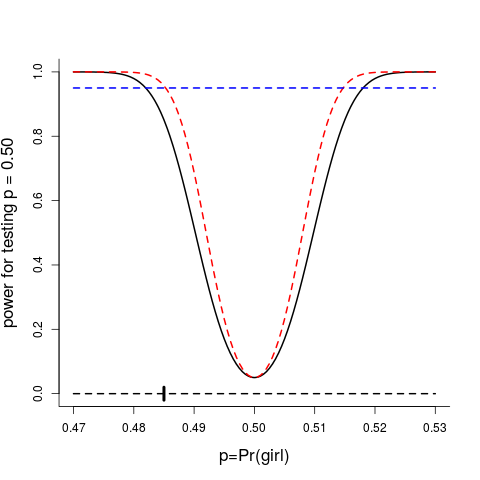
^{The power function, the probability of claiming that the true $p$ is not equal to $p_0=0.50$, as a function of $p$, plotted for $n=10000$ (black curve) and for $n=15000$ (red curve). At position $p_0$, the power is 0.05, the chosen significance level of the test, by construction.}

3. Children are extrabinomially overdispersed

The medical doctor Arthur Geißler (1832-1902, inside the reign of Königreich Sachsen, 1806-1918, making him perhaps a Saxon rather than a German, though Sachsen became part of the Deutsches Reich in 1871) was an eager collector of family and birth registry data, from all over Sachsen. Those were also the times of families with many children.

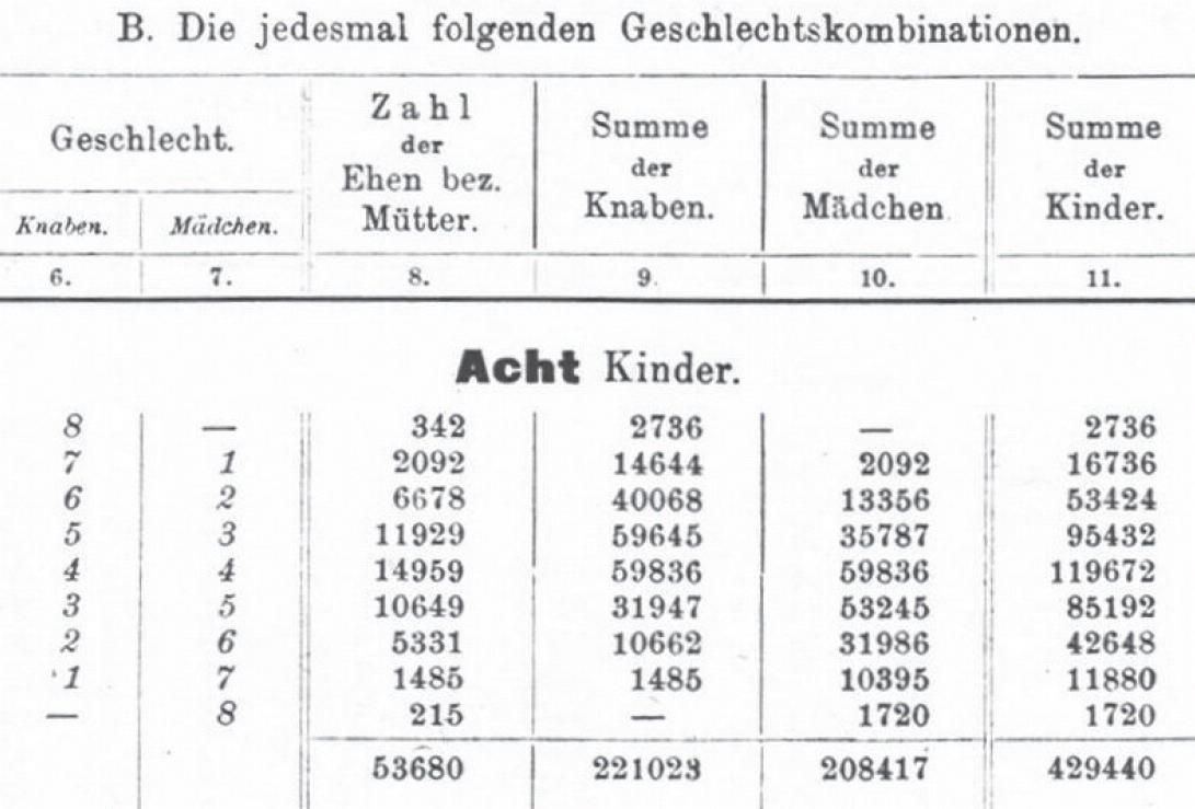
^{One of the tables in Geißler (1889), concerning families with eight children.}

From his collections of data tables, R.A. Fisher and others have extracted information on the number for girls, among the first $m=8$ children, for as many as $n=38495$ families, as follows, cf. Edwards (1958, 2005). So 264 had 0 girls, 1655 had 1 girl, 4948 had 2 girls, etc., see the first two columns in this table:

\(\matrix{ \def\ha{\phantom{-}} & &\hbox{binomial} & &\hbox{beta-binomial} & &\hbox{Markov} \cr y & N(y) & E_1(y) &\hbox{pears}_1 & E_2(y) &\hbox{pears}_2 & E_3(y) &\hbox{pears}_3 \cr 0 & 264 & 192.32 & \ha 5.17 & 255.54 & \ha 0.53 & 255.96 & \ha 0.50 \cr 1 & 1655 & 1445.38 & \ha 5.51 & 1656.79 & -0.04 & 1654.75 & \ha 0.01 \cr 2 & 4948 & 4752.36 & \ha 2.84 & 4909.50 & \ha 0.55 & 4906.78 & \ha 0.59 \cr 3 & 8498 & 8928.90 & -4.56 & 8683.46 & -1.99 & 8685.61 & -2.01 \cr 4 &10263 &10484.95 & -2.17 &10025.35 & \ha 2.37 & 10034.41 & \ha 2.28 \cr 5 & 7603 & 7879.79 & -3.12 & 7736.16 & -1.51 & 7734.77 & -1.50 \cr 6 & 3951 & 3701.20 & \ha 4.11 & 3896.34 & \ha 0.88 & 3893.65 & \ha 0.92 \cr 7 & 1152 & 993.42 & \ha 5.03 & 1171.05 & -0.56 & 1168.12 & -0.47 \cr 8 & 161 & 116.65 & \ha 4.11 & 160.81 & \ha 0.01 & 160.98 & -0.00 \cr & 38495 & 38495 & 159.41 & 38495 & 13.55 & 38495 & 13.17 \cr }\)

^{The Geißler (1889) data, for as many as $n=38495$ families with $m=8$ children, with $N(y)$ the number of these with $y$ girls, for $y=0,1,\ldots,7,8$. The table then gives the theoretical or expected number $E(y)$, for models (i) the binomial, (ii) the beta-binomial, (iii) the Markovian, see below, along with what I call Pearson residuals $(N-E)/\sqrt{E}$, The smaller these are, in absolute size, the better is the model behind them. The numbers 159.41, 13.55, 13.17 are the goodness-of-fit statistics, the sum of the squared Pearson residuals.}

So, out of $mn=307928$ children, $\sum_{y=0}^8 yN(y)=149158$ were girls (with $N(y)$ denoting the number of families with $y$ girls), leading to the overall estimate $\widehat p=0.484$ for the girl-probability. The third column gives the expected number

\(E_1(y)=nf(y,\widehat p)=n{m\choose y}\widehat p^y(1-\widehat p)^{m-y} \)

of the $n$ families with $y$ girls, for $y=0,1,\ldots,8$, under binomial circumstances. The fit is not so bad, though not in the category of `good', as revealed by what I term Pearson residuals

\(P_1(y) = {N(y)-E_1(y)\over \sqrt{E_1(y)}} \)

for $y=0,1,\ldots,8$ (placed in the pearson$_1$ column). Under the conditions of the model, that there is a binomial mechanism governing the number of girls, with the same $p$, these Pearson residuals would be approximately standard normally distributed, and with values outside the range $(-2.5,2.5)$ signalling that the fit is not good. Also, under model conditions, the goodness-of-fit statistic $Z_1=\sum_{y=0}^8 P_1(y)^2$ should have a $\chi^2_7$ distribution (a chi-squared with degrees of freedom equal to 7, the number of cells minus 1 minus another 1 for the number of parameters estimated); here $Z_1=159.82$, which is far too big.

So something is rotten in the state of Binomialia: the terrain has more weight at the borders ($y=0,1,7,8$) and less near the middle, compared to what the theoretical map predicts. The real world of the real children thus exhibits more variability than what a single binomial $p$ can explain. To shed light on this overdispersion, assume now that each family has its own girl-probability $p$ (whether this is due to the mother or the father, or to their con-divine conjunction habits), but that these vary from family to family, following some distribution $g(p)$, say. For each family we then have the well-known formulae

\({\rm E}\,(y\,|\,p)=mp \quad {\rm and} \quad {\rm Var}\,(y\,|\,p)=mp(1-p)\)

for the mean and variance. Let further $p_0$ and $\sigma_0$ be the mean and standard deviation of the background distribution of $p$ in the population of families. Then, using the laws of total mean and total variance (cf. the double expectation formula), we find

\({\rm E}\,y=mp_0 \quad {\rm and} \quad {\rm Var}\,y=mp_0(1-p_0)+m(m-1)\sigma_0^2\)

for the mean and variance of what Geißler and we actually observe in the population. So $m(m-1)\sigma_0^2$ is the extrabinomial variation, with a small $\sigma_0$ corresponding to the distribution of $p$ values being tight around its mean $p_0$. Note that with $m=1$, a land of one-child families, there is no such extrabinomial variation.

So let us assess the extra variation. Estimating $\sigma_0$ is not entirely straightforward, since it is the standard deviation of a variable we never actually observe, only indirectly, via the girl-counts $y_i$ themselves. We may however estimate the variance of the $y_i$ in the usual fashion, via

\(S_n^2={1\over n-1}\sum_{i=1}^n(y_i-\bar y)^2 ={1\over n-1}\sum_{y=0}^m N(y)(y-\bar y)^2,\)

with $\bar y=(1/n)\sum_{y=0}^m N(y)y=3.875$ the overall average number of girls, associated also with $\widehat p_0=\bar y/m=0.484$, and then subtract the binomial variance part, i.e. $m\widehat p_0(1-\widehat p_0)$. This difference, which turns out to become $2.1605-1.9981=0.1624$, is an estimate of $m(m-1)\sigma_0^2$. Dividing with $8\cdot7$ and taking the square root yields $\widehat\sigma_0=0.0539$, indicating that about 95% of the families of the world (at least in Sachsen, in the late 19th century) have their $p$ inside $[0.38,0.58]$ – I provide a more accurate assessment below.

We ought to provide a clear statistical test for the presence of overdispersion. A natural test statistic is

\(W_n={S_n^2\over m\widehat p_0(1-\widehat p_0)},\)

since this ratio will be close to 1 under fixed $p$ circumstances but bigger than 1 in the presence of a positive $\sigma_0$. Here we find $W_n=1.081$, which might not look impressive, but is; the 0.01 and 0.99 quantiles of the null distribution of $W_n$, based on $10^4$ simulations under binomial conditions, are 0.984 and 1.016.

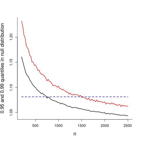
I pause briefly to comment on how the sample size influences both p-values and detection power. Observing the full-variance to under-model-variance ratio $W_n=1.081$ is found to be superconvincing evidence for overdispersion here, due to $n$ being so large; with a smaller $n$ it might not qualify as significant. The figure below displays the 0.95 quantile (black) and 0.99 quantile (red) in the null distribution of $W_n$, as a function of sample size. So the observed value 1.081 starts getting interesting at around $n=750$ (p-value below 0.05) and very convincing at around $n=1500$ (p-value below 0.01); and, of course, with $n=35000$ or more, as with the Sachsen data, the null hypothesis associated with the pure binomial is blown away.

4. A better model: the beta-binomial

A very reasonable model to try out is to place a ${\rm Beta}(a,b)$ distribution on the $p$, with density say $g(p,a,b)$. The distribution of the girl-count $y$ in a family of $m$ children then takes the form

\(\eqalign{ f_2(y,a,b)&=\int_0^1 f(y,p)g(p,a,b)\,{\rm d}p \cr &=\int_0^1{m\choose y}p^y(1-p)^{m-y} {\Gamma(a+b)\over \Gamma(a)\Gamma(b)} p^{a-1}(1-p)^{b-1}\,{\rm d}p \cr &={m\choose y}{\Gamma(a+b)\over \Gamma(a)\Gamma(b)} {\Gamma(a+y)\Gamma(b+m-y)\over \Gamma(a+b+m)}, \cr}\)

for $y=0,1,\ldots,m$. The parameters $(a,b)$ can be fitted via maximum likelihood, by minimum chi-squared, or by equating the observed mean $\bar y$ and variance $S_n^2$ to the corresponding population quantities

\({\rm E}\,y=mp_0=m{a\over a+b}\)

and

\({\rm Var}\,y=mp_0(1-p_0)+m(m-1)\sigma_0^2 =mp_0(1-p_0)+m(m-1){p_0(1-p_0)\over a+b+1}.\)

This moment estimation method leads directly to $\widehat p_0=\bar y/m=0.484=a/(a+b)$ again, and a simple equation for finding $a+b$.

These three estimation approaches give rather similar results for the 8-children families from 19th century Sachsen. The minimum chi-squared method consists in minimising the sum of the Pearson residuals

\(Q_n(a,b)=\sum_{y=0}^8 P_2(y)^2 =\sum_{y=0}^8 \{N(y)-E_2(y,a,b)\}^2/E_2(y,a,b) \)

over all $(a,b)$, where $E_2(y,a,b)=nf_2(y,a,b)$ is the expected number of families with $y$ girls, under the model being studied. I find $(\widehat a,\widehat b)=(41.179,43.833)$, amounting to a Beta density with mean 0.484 and standard deviation $\sigma_0=0.0538$. So 95% of all couples have their $p$ inside the interval $[0.396,0.573]$. That the fit of the beta-binomial is very good is seen via the table above, with fits $E_2(y,\widehat a,\widehat b)$ close to the observed counts $N(y)$, with Pearson residuals $P_2(y)$ within the standard normal range, in total offering a drastic improvement on the simple binomial fixed-p explanation. The minimum sum of squares $Z_2=Q_n(\widehat a,\widehat b)=13.721$ is admittedly not entirely perfect, compared to the scale of the $\chi^2_6$ (now with degreees of freedom equal to 6, namely the number of cells minus 1 minus 2 more for the two estimated parameters), but taking the enormous Saxonic sample size of $n=38495$ into account the statistician really can't ask for a better fit.

The size of the extrabinomial dispersion is of particular interest, i.e. the standard deviation $\sigma_0$ in the distribution of $p$ across a broad population of families. I've gone to the trouble of computing a confidence curve ${\rm cc}(\sigma_0)$ for this parameter, using methods of Schweder and Hjort (2017, Chs. 3-4), as follows.

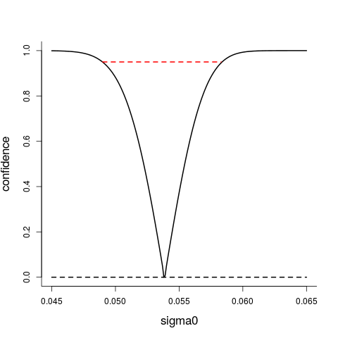
^{The confidence curve ${\rm cc}(\sigma_0)$ for the overdispersion parameter $\sigma_0$; the point estimate is 0.0538 and the 95% interval is $[0.0490,0.0583]$.}

5. Markovian children

For the Geißler data we do not have information of the order of girls and boys, just their totals. A fascinating data set analysed in Kotz (1972) has however order information, for each of a high number of Amish and Mennonite families, with parents born before 1910. This is from the era where birth control was considered sinful and with `be fruitful and multiply' ruling. He fitted these binary sequences to a Markov model, estimating a certain association parameter, and found this to be just visible, as in barely significant. In connection with writing up this blogpost I have accessed these data and worked with them myself (where a serious and time-consuming challenge, for me, was to translate the octogonal coding of Kotz's data back to understandable binary sequences). I have also confirmed that the Markov dependence, in the model he set up, is just about visible for the data, but not in a prominent fashion.

I was curious enough to fit also the Geißler data to a natural Markovian model. This takes further efforts, since I only know that you have $y$ girls and $m-y$ boys, not the order or the $m$ children. Hence I cannot use the machinery of Kotz (1972, 1973), but as long as I put up a parametric model for $x_1,\ldots,x_m$, with $x_i=1$ for girl and $x_i=0$ for boy, I can for any $\theta$ in that model simulate a large number of gender paths $x_1,\ldots,x_m$, read off the number of girls $y=\sum_{i=1}^m x_i$, and estimate say $f_3(y,\theta)$, the implied distribution, by checking the proportion of paths which led to $y$. In particular, I can compute (well, actually, simulate good enough approximations to) and work with the log-likelihood function

\(\ell(\theta)=\sum_{i=1}^n\log f_3(y_i,\theta)=\sum_{y=0}^m N(y)\log f_3(y,\theta),\)

even when there is no explicit formula for $f_3(y,\theta)$. This the approach of simulated log-likelihood, obtaining an estimate $\widehat\ell(\theta)$ through simulation, for a grid of $\theta$ values.

Let me now introduce my model for the Markovian children, where the gender of your next child depends (but only slightly, as it turns out) on the gender of your currently last child. Let $(q_0,p_0)=(1-p_0,p_0)$ be the long-term frequencies for boys and girls. Instead of taking births to be fully independent of each other, consider the Markov chain $x_1,x_2,\ldots$ of births (again with 0 for boy and 1 for girl), with $x_1$ drawn from the $(q_0,p_0)$ coin of things, and then following the two-stage transition probability matrix

\(P=\pmatrix{1-kp_0 & kp_0 \cr kq_0 &1-kq_0}, \)  

with $k$ a fine-tuning parameter. If $k=1$ we're back to ordinary independence, with $(q_0,p_0)$ for each new birth. This Markov chain has $(q_0,p_0)$ as its equilibrium distribution. The covariance beetween consecutive "it's a girl" and "it's a girl" is

\(p_0(1-kq_0)-p_0^2=p_0q_0(1-k)\)

so the correlation between girl, girl is $1-k$; the same expression is also valid for the correlation between boy, boy. We shall find $k$ around 0.95 below, which then means "same gender twice" correlation around 0.05.

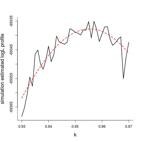
With considerable efforts I have fitted this two-parameter Markov model to the Geißler data, for the case of $m=8$ as well as for the other family sizes (see below for these data). This involves somewhat heavy simulations, constructing figures as the one below, zooming in via the right grids, etc. For my favourite case of $m=8$, I find $\widehat k=0.956$, with 99% interval $[0.947,0.964]$, which means correlation between (girl, girl), or between (boy, boy), estimated at 0.044 with interval $[0.036,0.053]$.

The fit of this after all relatively simple Markov model is remarkably good, as seen in the two last columns of the table in Section 3. The view taken for this model is that the same parameters $(k,p_0)=(0.956,0.484)$ are at work across all families, with transition matrix

\(\widehat P=\pmatrix{0.537 & 0.463 \cr 0.492 & 0.508 \cr}\)

governing the next child's gender. The minimum chi-squared statistics is 13.17 (found via an embarrassingly high number of simulations, to make it precise enough), just a bit smaller than than for the beta-binomial. I've also gone to the considerable trouble of computing the maximum log-likelihood value (again, via simulations) for the Markov model, comparing this with the corresponding value for the beta-binomial model, for each of the family sizes $m=2,3,\ldots,12$. These numbers are needed for model comparisons and ranking via the model selection criteria AIC or BIC (see Claeskens and Hjort, 2008). The two models are quite comparable. Focused categorical model selection via FIC methods in Hjort and Jullum (2018) may also be brought to the table, when special questions, like estimating the probability of all-girls families, are under consideration. 

One may also extend the initial Markov model above a bit further, to improve the fit a tad or two more, e.g. by allowing a distribution for the $p_0$ while keeping the Markov parameter $k$ fixed. This can be done using the methods developed above, but with added efforts (model building, programming, interactive simulations).

6. Are the sex ratio and the overdispersion level changing with family size?

I have excerpted the following table of information from related data summaries in Edwards (1958) and Lindsey and Altman (1998), who again have used the Sachsen 1889 tables to provide counts of $y$ girls in families of $m$ children, for $m=1,2,\ldots,12$. So there were 6115 families with 12 (or more) children, with the girl probability estimated to $\widehat p=35280/(12\cdot6115)=0.481$ for these, etc.

\(\matrix{ &m &0 &1 &2 &3 &4 &5 &6 &7 &8 &9 &10 &11 &12 \cr G01 & 1 &114609 &108719 & \cr G02 & 2 & 47819 & 89213 &42860 \cr G03 & 3 & 20540 & 57179 &53789 &17395 \cr G04 & 4 & 8628 & 31611 &44793 &28101 & 7004 \cr G05 & 5 & 3666 & 16340 &30175 &28630 &13740 &2839 \cr G06 & 6 & 1579 & 7908 &17332 &22221 &15700 &6233 &1096 \cr G07 & 7 & 631 & 3725 & 9547 &14479 &13972 &8171 &2719 & 436 \cr G08 & 8 & 264 & 1655 & 4948 & 8498 &10263 &7603 &3951 &1152 &161 \cr G09 & 9 & 90 & 713 & 2418 & 4757 & 6436 &5917 &3895 &1776 &432 & 66 \cr G10 &10 & 30 & 287 & 1027 & 2309 & 3470 &3878 &3072 &1783 &722 &151 & 30 \cr G11 &11 & 24 & 93 & 492 & 1077 & 1801 &2310 &2161 &1540 &837 &275 & 72 & 8 \cr G12 &12 & 7 & 45 & 181 & 478 & 829 &1112 &1343 &1033 &670 &286 &104 &24 &3 \cr }\)

^{The table gives the number of Sachsen families, sorted by family size, with a given number of girls. Thus the line G08 relates to the $264 + 1655 + \cdots + 1152 +161 = 38495$ families we've met earlier, with $m=8$ children, and with the 9 columns indicating the number of these with $y=0,1,\ldots,8$ girls, and similarly for the other rows.}

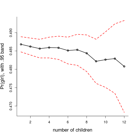
Using the methods above I can patiently go through each family size, $m=1,2,\ldots,12$, and estimate and assess $p_0$ and the extrabinomial variation parameter $\sigma_0$ for each. This leads first to this figure, with the $\widehat p_0$, along with a 0.95 pointwise confidence band. Yes, the $p=P(\hbox{girl})$ appears to climb a little bit down, but this is not significant. You may still fit your horizontal ruler inside the band, and a proper test for the null hypotheses that the twelve $p_m$ are identical does not signal anything wrong, even with the enormous sample sizes involved. So here I carefully disagree with claims made by Edwards (1958) and Lindsey and Altham (1998).

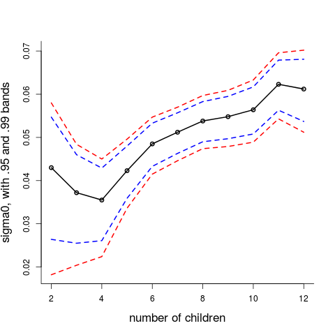
What is however clear from these data is that the level of extrabinomial dispersion increases with the bigger families, as seen in this figure, where I've used the confidence curves machiney of Schweder and Hjort (2016) to calculate 0.95 and 0.99 intervals for $\sigma_0$, for each family size. What we've learned above is that there might be several competing reasons for this overdispersion. It could be that the $p$ varies even more across families of size $m=10$ than for those of size $m=5$, etc., or there could be dependencies in the chains of genders, and one might think of yet more involved tiny mechanisms. These would all be small (if they had been big, humans studying humans would have noticed them much more easily), but it is again part of this story of stories that with such enormous sample sizes the statistical microscopes can pick up even tiny effects and discrepancies from what we might think of as Nature's default operations.

7. Concluding comments

A: The quality of the Geißler (1889) data. Let me first point to an important detail I chose to pass over above: when I discuss data for "families with 8 or more children", etc., these actually have 9 or more children, with Geißler and later writers having been careful enough to remove the gender of the ninth child from his tables, in order not to disturb the study of the human sex ratio via some present or imagined "stopping rules". So the tables above, with $y$ girls out of $m$ children, pertain to the first $m$ children in families with at least $m+1$ children. 

Certain concerns have been voiced regarding the quality and relative cleanliness of the Geißler data, which apparently contain a certain but low number of repetitions, etc. Generally the data quality is judged good enough to yield good statistical analyses of the real gender producing processes, however; cf. Edwards (1958, 2005). This is also my viewpoint (after having checked Edwards's points), in particular for the work I've carried out in this blog post.

B: How many 8-children families must I check out before I spot the extrabinomial variance? I showed above that we need to check the gender of some 10000 or ideally even 20000 children to really be statistically fully certain that $p=P(\hbox{girl})$ is not 0.50, but a bit below 0.49. I've also commented that the p-value associated with having computed the total-variance to model-variance ratio $W_n=1.081$ test, for testing the null hypothesis that the pure binomial is correct, depends on the sample size, i.e. the number $n$ of families with $m=8$ children in the dataset. With $n=1500$, the p-value becomes very convincing, but not for e.g. $n=500$.

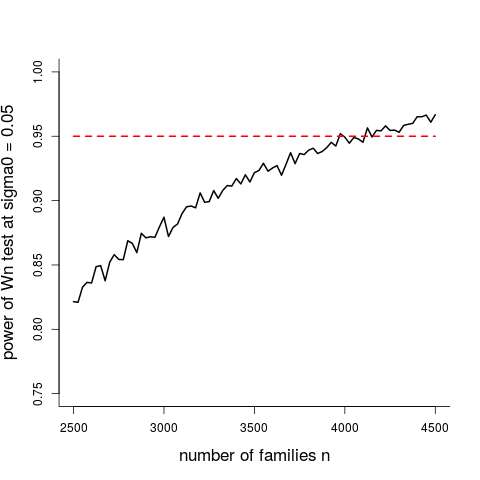
We may also ask how big $n$ ought to be before the statistical power of the $W_n$ test is above level 0.95, say, if the true state of affairs corresponds to the $\sigma_0=0.05$ (I estimated this extrabinomial standard deviation parameter to be $\widehat\sigma_0=0.0538$ above). The figure below answers this question. It provides the power of the $W_n$ test, calibrated to have significance level 0.05, at that position in the alternative space where $\sigma_0=0.05$, as a function of the number $n$ of families. I have done this via simulating $10^4$ realisations of $W_n$ at the null model, to identify the rejection level, and then simulating another $10^4$ realisations of $W_n$ at the alternative position, checking how often the test rejects the null. We learn that about $n=4000$ families of size $m=8$ children are required for the careful statistician to be satisfied.

C: The over-representation of all-girls and all-boys. So among the $n=38495$ families with $m=8$ children, there were 264 with all-boys and 161 with all-girls. These numbers are a bit bigger than what the binomial view of the world would predict, namely 192 and 117. With the beta-binomial model I can compute the theoretical over-representation ratios for all-boys and for all-girls, as follows.

\(\matrix{ m &\hbox{all boys} &\hbox{all girls} \cr 2 & 1.007 & 1.008 \cr 3 & 1.016 & 1.018 \cr 4 & 1.029 & 1.032 \cr 5 & 1.068 & 1.077 \cr 6 & 1.137 & 1.155 \cr 7 & 1.217 & 1.247 \cr 8 & 1.329 & 1.379 \cr 9 & 1.452 & 1.535 \cr 10 & 1.636 & 1.762 \cr 11 & 2.059 & 2.256 \cr 12 & 2.223 & 2.522 \cr }\)

^{The table gives the over-representation ratios for all-boys families, $E_2(0)/E_1(0)$, and for all-girls, $E_2(m)/E_1(m)$, among families with $m$ children.}

D: Yet other models. Of course other models for the machineries of nature can be put forward, fitted to these data, and compared; see e.g. Lindsey and Altham (1998) for a couple of proposals. It would also be natural to use model selection tools, as with the AIC, the BIC, the FIC (cf. Claeskens and Hjort, 2008, Hjort and Jullum, 2018), to rank different models.

E: Yet other data. Nichols (1905) discusses an interesting dataset with about 3000 families, with 6 or more children, mostly of Anglo-Saxon descent, from the 1600-1850 era. His conclusions appear to match those obtainable from Geißler (1889), regarding the basic probability parameter $p=P(\hbox{girl})$.

F: Are more boys being born during wars? This question has been raised in the past, but as far as I've understood it has been dismissed as a small statistical fluke, with apparent bumps in some graphs within reasonable stationary fluctuations after all. However, Sir David Spiegelhalter (2015a, 2015b) comes to the rescue, and finds that the old myth is not a myth, but the Real Thing, complete with a reasonable statistical argument (related to random visits inside the menstrual cycles).

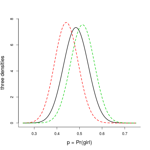
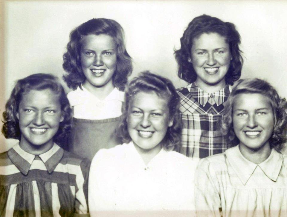
G: Assessing p after all the births. The figure displays three Beta densities for $p=P({\rm girl})$. The black in the middle is the overall one, valid in the population at large, with parameters $(a,b)$ as estimated above. The red to the left is for Kristin Lavransdatter, with parameters $(a,b+8)$; as we recall from reading the Nobel Prize 1928 classic, she and Erlend Nikulausson had eight sons: Naakve, Bjørgulf, Gaute, Ivar, Skule, Lavrans, Munan, and Erlend. The green to the right must be for Nils Lid and Dagny Fosse, with parameters $(a+5,b)$, as per the intro photo.

References

Arbuthnot, J. (1710). An argument for Divine Providence, taken from the constant regularity observ'd in the births of both sexes. Philosophical Transactions, vol. 27, 186-190.

Claeskens, G. and Hjort, N.L. (2008). Model Selection and Model Averaging. Cambridge University Press.

Edwards, A.W.F. (1958). An analysis of Geissler's data on the human sex ratio. Annals of Human Genetics, vol. 23, 6-15.

Edwards, A.W.F. (2005). Sexes and statistics. Significance, vol. 2, issue 4, 185-186.

Fisher, R.A. (1930). The Genetical Theory of Natural Selection. The Clarendon Press, London.

Geißler, A. (1889). Beiträge zur Frage des Geschlechts verhältnisses der Geborenen. Zeitschrift des königlichen sächsischen statistischen Bureaus, vol. 35, 1-24.

Hjort, N.L. and Jullum, M. (2018). Categorical model selection. Manuscript in preparation.

Klotz, J. (1972). Markov chain clustering of births by sex. Proceedings of the Sixth Berkeley Symposium on Mathematical Statistics, vol. 4, 173-185.

Klotz, J. (1973). Statistical inference in Bernoulli trials with dependence. Annals of Statistics, vol. 1, 373-379.

Lindsey, J.K. and Altham, P.M.E. (1998). Analysis of the human sex ratio by using overdispersion models. Applied Statistics, vol. 47, 149-157.

Nichols, J.B. (1905). The sex-composition of human families. American Anthropologist (New Series), vol. 7, 24-36.

Schweder, T. and Hjort, N.L. (2016). Confidence, Likelihood, Probability: Statistical Inference With Confidence Distributions. Cambridge University Press, Cambridge.

Spiegelhalter, D. (2015a). Sex-rated statistics. Significance, vol. 12, issue 4, 21-25.

Spiegelhalter, D. (2015b). Sex by Numbers: What Statistics Can Tell Us About Sexual Behaviour. Wellcome Collection, London.

Stigler, S. (1986). The History of Statistics: The Measurement of Uncertainty Before 1900. Harvard University Press.

Waaler, G.H.M. (1928). Om seksualproportionen ved födslen. Nordisk Statistisk Tidsskrift, vol. 7, 65-69.