
[Tore Schweder is a frequent collaborator with Nils Lid Hjort and an active friend of the FocuStat group and project. We've invited him to give us a guest blog post, qua gjesteskribent. An earlier and rather shorter version of this story has appeared in Tilfeldig Gang, juni 2017.]
To illustrate differences in approach and sometimes in conclusion, I consider the following dataset, pertaining to macro-economics of the USA over the years 1929 to 1940, on
- consumption (C),
- investment (I),
- government spending (G),
with the unit being one billion 1932 dollars. The data have been used by Christopher Sims, recipient of Sveriges riksbanks pris i ekonomisk vetenskap till Alfred Nobels minne, for 2011 (and I'm grateful to Sims for sending me the data). The question focused on by Sims is how much growth in consumption affects investment. Denote by \(\theta_1\)this effect size. The statistical task is inference for this parameter.
| year | I | G | C |
| 1929 | 101.4 | 146.5 | 736.3 |
| 1930 | 67.6 | 161.4 | 696.8 |
| 1931 | 42.5 | 168.2 | 674.9 |
| 1932 | 12.8 | 162.6 | 614.4 |
| 1933 | 18.9 | 157.2 | 600.8 |
| 1934 | 34.1 | 177.3 | 643.7 |
| 1935 | 63.1 | 182.2 | 683.0 |
| 1936 | 80.9 | 212.6 | 752.5 |
| 1937 | 101.1 | 203.6 | 780.4 |
| 1938 | 66.8 | 219.3 | 767.8 |
| 1939 | 85.9 | 238.6 | 810.7 |
| 1940 | 119.7 | 245.3 | 752.7 |
The model, which the Bayesian and the frequentist agree on here, is of a type going back to Trygve Haavelmo (winner of the same not-quite-Nobel-Prize in 1989), with three macro-economic time series satisfying a simultaneous linear equations model with normally distributed errors. With $Y_t=C_t+I_t+G_t$, the model is
\(\eqalign{ C_t &= \beta+\alpha Y_t+\sigma_C Z_{1,t}, \cr I_t &= \theta_0+\theta_1(C_t-C_{t-1})+\sigma_I Z_{2,t}, \cr G_t &= \gamma_0+\gamma_1 G_{t-1}+\sigma_G Z_{3,t}. \cr}\)
It has five non-zero coefficients in addition to $\theta_1$, along with three standard deviation parameters $\sigma_C,\sigma_I,\sigma_G$, and the $Z_{j,t}$ are independent standard normals. To estimate the parameter in focus, the Bayesian needs a prior distribution for all the six linear parameters in addition to the three variances. This distribution must be based on knowledge or judgments and should not depend on the observed 1929-1940 data. By combining the prior distribution and the statistical model a posterior distribution for $\theta_1$ is obtained by Bayes' formula -- which here is a non-trivial computational exercise in setting up a Markov Chain Monte Carlo scheme.
(Well, Sims, it's not the Nobel Prize.)
Christopher Sims used this example to demonstrate the virtues of the Bayesian methodology when he received the Sveriges Riksbank Prize in Economic Sciences in Memory of Alfred Nobel for 2011. He chose to use flat and independent prior densities for the six coefficients and for the logarithm of the error variances. The parameter of interest, $\theta_1$, is assumed positive.The prior distribution is not a probability density since its density integrates to infinity. It is chosen to not colour the posterior distribution much. The posterior distribution for $\theta_1$ turns out to have most of its mass somewhat close to zero (but with zero posterior point-mass at zero itself). The posterior cumulative distribution function is shown in the figure (which is slightly more polished and accurate than the one we used in CLP, Ch 14).
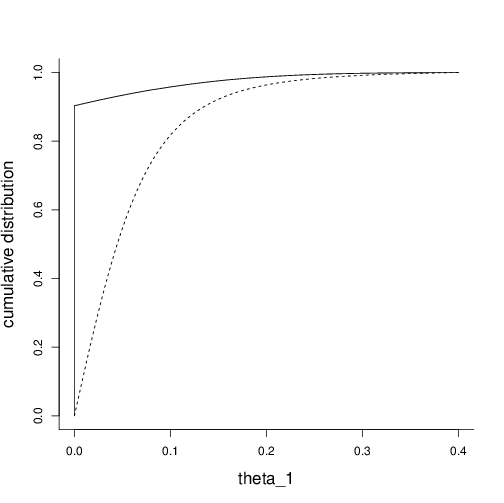
Figure: The cumulative confidence distribution for $\theta_1$ (full black) together with an approximation to the cumulative posterior distribution obtained by Sims (2012) (dotted line).
The choice of prior distribution does necessarily colour the Bayesian posterior distribution. There is actually no such thing as a fully noninformative prior. For this and additional reasons discussed in Schweder and Hjort (2016, Ch 14) I do not agree with Sims (2007), who claimed `Bayesian Methods in Applied Econometrics, or, Why Econometrics Should Always and Everywhere Be Bayesian'.
Difficuties with setting up noninformative priors contributed to pushing R.A. Fisher to develop the method of fiducial probability (Fisher, 1930). The other giant frequentist statistician, Jerzy Neyman, used a fiducial probability distribution to obtain confidence intervals. If 90% of the fiducial probability is within the interval (a, b), then this is a 90% confidence interval. The modern notion of a confidence distribution is that an interval holding a fraction $p$ of the total confidence is a confidence interval of degree $100p\%$ for all $ 0 \leq p \leq 1$. This amounts to the confidence to the left of the true value of the parameter being uniformly distributed in repeated sampling.
In simple models confidence distributions are obtained by Fisher's fiducial distribution. As with Bayesian posteriors, simulations are however usually required. Schweder and Hjort (2016) give a book length treatment of confidence distributions and confidence curves, with many examples, including the one discussed here.
Confidence distributions are often close to Bayesian posterior distributions. But for small samples and models with restrictions, such as in the example discussed here, there might be a difference. I've changed Sims' model slightly by assuming $\theta_1 \ge 0$ rather than $\theta_1 >0$. Otherwise data and model are the same. The resulting cumulative confidence distribution is also displayed in the figure. The confidence distribution has a point mass of 0.9003 at zero, and the rest spread out on small positive values. We are actually 99% confident that $\theta_1 \leq 0.286$.

Sims (left) is challenged in this blog post.
Confidence is really epistemic probability (Schweder, 2017). In view of the data and the model there is about 90% probability that $\theta_1=0$ and 99% that it is less than 0.286. Sims agrees that with about 99% probability the parameter is less than 0.29, but distributes this probability continuously over the interval to the right of the confidence distribution. The prior distribution does actually pull the Bayesian distribution to the right of zero. My result is obtained without any prior input other than the data and the statistical model, and I claim that the confidence distribution reflects better than the Bayesian posterior our knowledge and its surrounding uncertainty about the effect upon investments of a yearly change in consumption, $\theta_1$, in USA, in the decade before the war.
References (with more in the CLP book; check in particular its application chapter 14):
Fisher, R.A. (1930). Inverse probability. Proceedings of the Cambridge Philosophical Society, 26, 528-535.
Haavelmo, T. (1943). The statistical implications of a system of simultaneous equations. Econometrics, 11, 1-12.
Schweder, T. and Hjort, N.L. (2016). Confidence, Likelihood, Probability: Statistical inference with confidence distributions. Cambridge University Press.
Schweder, T. (2017). Confidence is epistemic probability for empirical science. Journal of Statistical Planning and Inference.
Sims, C.A. (2007). Bayesian methods in applied econometrics, or, why econometrics should always and everywhere be Bayesian. Hotelling lecture.
Sims, C.A. (2012). Statistical modeling of monetary policy and its effects [Nobel Prize Lecture in Economics]. American Economic Review, 102, 1187-1205.
Log in to comment
Not UiO or Feide account?
Create a WebID account to comment