
- Producing a simple document
- Setting parameters
- Document and page organisation
- Pagebreaks, space, footnotes, references, boxes, etc
- Special characters
- Environments
- Scaling, rotation, clipping, wrap-around and shadows
- Maths
- Special characters
- Fonts
- Examples
- Environment variables
Using LaTeX on linux machines:
To load the paths (TexLive):
module load texlive
Producing a simple document
Writing LaTeX
It is very easy to use LaTeX to produce simple documents containing text with occasional headings. You put :
\documentclass[12pt]{article}
\usepackage{a4}
\begin{document}
at the top and
\end{document}
at the end. If you want to have numbered section headings in the text use the command
\section{This is the Text of the Heading}
If you don't want the numbering, use \section* instead of \section. The text of the document is just typed in as normal except that each time you want to start a new paragraph you should leave a blank line.
There are a small number of characters which have special meanings in LaTeX so if you need to use them they will need to be entered specially into your file. The characters are:
& $ # % _ { } ^ ~ \
If you really need any of the first seven of these they can be inserted by typing the two character combinations shown below.
\& \$ \# \% \_ \{ \}
The `\' character is used in each case to tell LaTeX that the character that comes next should not have its special meaning in this case. When you are happy with the document, save it. There's no need to shut down the editor.
Processing LaTeX documents
To process your LaTeX document type:
> latex mydoc.tex
If an error occurs, details will be given of the line in which the error was detected. Try to correct the error in your Editor window and process again. Note also that LaTeX produces several files which you normally do not need to worry about (.aux, .toc, .lof, .lot, .log).
When LaTeX has processed your document successfully you will be left with a number of new files, all with the same base name as your original, but having different suffices. The one we are interested in is the `.dvi' file. This file shouldn't be viewed using emacs, but can be looked at using the xdvi previewer, type:
> xdvi mydoc.dvi
You can use the mouse to magnify bits of the window. Just press a mouse button over the part of the text you want to see in more detail. The middle button works the scroll bars. Click on the buttons to the right of the window to move around the document.
To print your document you need to convert it to PostScript (which may also be viewed with ghostview) and send the resulting PS-file to the printer. To convert a .dvi file to PostScript and print it, type:
> dvips mydoc.dvi
This is dvips 5.490 Copyright 1986, 1992 Radical Eye Software
' TeX output 1998.10.02:1835' -> mydoc.ps
> tex.pro>. [1] [2] [3] [4] [5] [6] [7]
> ppr mydoc.ps
The relevant programs used in processing LaTeX documents are listed in the table below:
| Program | Description |
|---|---|
| latex | the LaTeX processing program |
| xdvi | a DVI file previewer |
| dvips | a DVI-to-PS converter |
| dvipdf | a DVI-to-PDF converter |
Setting parameters
Counters
LaTeX maintains many counter variables (e.g. page, part, equation, footnote, chapter, paragraph, section, subsection, subsubsection, enumi, etc). You can set these counters yourself. Some examples :
\setcounter{page}{0}
\addtocounter{chapter}{2}
Length parameters
LaTeX accepts the following units of length: in, cm, mm, pt (there are 72.27 pts to an inch), em (width of an M), ex (height of an x). These units can be used to set the values of length variables using \setlength. For example,
\setlength{\parindent}{0in}
sets to zero the amount by which the first line of a paragraph is indented. Other useful length parameters are :
- parskip: determines the gap between paragraphs.
- baselineskip: determines the usual distance from the bottom of one line to the bottom of the next. You can adjust this to produce double spacing, but a better way, which takes a stretch factor as argument is to use \linespread. For instance before \begin{document} you can do \linespread{1.6} to get doublespacing through your document. The setspace package offers more options.
Document and page organisation
Document classes
The standard classes are article, book, letter, report, slides. The differences between these are often minor. A book can have chapters. In a report sections begin at 0 whereas in an article they begin at 1.
Big Documents
It's best to split your document into smaller files and have a master file looking like this
\documentclass[dvips,12pt]{book}
\usepackage{a4,color,graphics,palatino,fancyhdr}
\begin{document}
\pagestyle{empty}
\tableofcontents
\listoffigures
\pagestyle{fancy}
\appendix
\end{document}
on which you can run latex just as if the master file contained all the text of chapter1.tex etc. The advantage of this is that once you have a chapter correct, you can comment out the corresponding `input' line and avoid unnecessary processing. Remember to take out the \begin{document} and \end{document} lines from the component files.
Page Size
You can choose the margin sizes yourself by changing the following dimensions before the \begin{document} line.
\setlength{\topmargin}{-0.4in}
\setlength{\topskip}{0.3in}    % between header and text
\setlength{\textheight}{9.5in} % height of main text
\setlength{\textwidth}{6in}    % width of text
\setlength{\oddsidemargin}{0.75in} % odd page left margin
\setlength{\evensidemargin}{0.75in} % even page left margin
Note that a margin width of 0cm gives you a margin 4cm wide. Rather than set absolute sizes you can modify the default sizes using commands like the following -
\addtolength{\evensidemargin}{-1cm}
\addtolength{\oddsidemargin}{-1cm}
\addtolength{\textwidth}{2cm}
Further support for control of page layout is provided by the geometry package. To see the current values of these dimensions, use the layout package, which defines a \layout command.
For A3 output, add \usepackage{a3} to your latex source file, run latex on it, convert the resulting file to Postscript using "dvips -t a3 foo.dvi -ofoo.ps" then print using "ppr -XHP5_TRAY=a3 -Pastro foo.ps".
Title Pages
The title page of a document is set before \begin{document} using the following commands :
\title{Intro to \LaTeX}
\author{A. O. Jaunsen}
\date{\today}
\maketitle
Contents
Use \tableofcontents to create a contents list at that point in the document. LaTeX will pick out the sections, subsections etc for you. You'll have to run LaTeX at least twice though.
Page numbers and headings
These are determined by the argument given in pagestyle{}.
- plain: the page numbers are put at the bottom of the page. The top of the page is empty. This is the default mode.
- empty: this suppresses page numbering altogether, except on the title page it you're using \maketitle. The workaround in this case is to do
\maketitle
\thispagestyle{empty}
with no gap between the two lines.
- headings: this puts the page numbers at the top and adds a header whose contents depend on the document style.
fancyhdr is a popular package that adds useful page headers when \pagestyle{fancy} is used.
Long section titles can cause trouble in headers. The section commands let you specify an extra, shorter title for use in the header and contents page, for example :
\subsection[Pagebreaks, footnotes, etc]
   {Pagebreaks, space, footnotes, references, boxes, etc}
Sectioning
To start a chapter called Life in a book, just use \chapter{Life}. Similar commands to start a part, section or subsection also exist in most document classes (articles don't have chapters or parts though). Here is a table of valid section-commands :
| Command | Note |
|---|---|
| \chapter | NOT in articles |
| \section | |
| \subsection | |
| \subsubsection\ | |
| \paragraph | |
| \part | NOT in articles |
If you use the *-form of the command then the sections will not be numbered, neither will it appear in the table of contents (eg. \section*{Life}).
A title will only be numbered if its 'depth' isn't more than secnumdepth and will only appear in the contents page if the 'depth' isn't more than the value of tocdepth. So, for example, doing
\setcounter{tocdepth}{2}
\setcounter{secnumdepth}{3}
will cause section 1.4.3 to be numbered, but it won't appear in the contents.
Pagebreaks, space, footnotes, references, boxes, etc
Page Breaks
You can force a page break using \newpage.
Preventing line breaks
If there's a word that you don't want broken, put it in an mbox. E.g., one shouldn't try to break up
\mbox\emph{relationships}
Space
You can create vertical space \vspace{.5cm} between lines or horizontal space \hspace{1.5cm} between words. The arguments to these commands can be negative. You can create vertical space between lines or horizontal space between words. The arguments to these commands can be negative. \vspace* will create space even at the top of a page. It's sometimes useful to create stretchable space. The following creates space that pushes the letters to the edge of the page
\noindent A\hspace{\stretch{1}} B\\
C\hspace{\stretch{1}} D
Footnotes
Do them like this
\footnote{I told you so.}
The footnotes are numbered by default. If you want to use symbols (stars, daggers etc) then you need to redefine how the footnote counter is displayed.
\def\thefootnote{\fnsymbol{footnote}}
Margin notes
Do them like this
\marginpar{margin note}
Cross References
At the end of this source file is the line
\label{THE_END}
\pageref{THE_END} will refer to the final page by number, and \ref{THE_END} will refer to it by section number. The last page (page 37 is in section 6.) You'll have to run LaTeX at least twice to pick up forward references like these.
Boxed Text
For short pieces of text, use \fbox
Help. I'm \fbox{trapped}

Comments
Anything to the right of a % character is ignored by LaTeX
Rules
The \rule takes 2 arguments; a width and a height, so \rule{\textwidth}{1pt} produces

Special characters
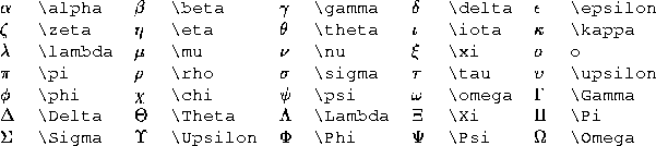
§ is created by \S, ¶ by \P, £ by \pounds, ö by \"{o}, © by \copyright. %" Many others are available in the math environment, including all the lower case greek letters and most of the upper case ones. If you only want to use a few characters you can bracket the symbols using $ and $ rather than \begin{math} and \end{math}. You can put a slash through any of these characters by prefacing them with \not.
Environments
Alignments
In these environments \\ starts a new line.
\begin{flushleft}
Some people like to stay firmly\\ on the left whereas others
\end{flushleft}
\begin{flushright}
feel much more at home\\ on the right.\\
\end{flushright}
\begin{center}
but most of us prefer to stay dead in the center.
\end{center}
Listing items
The items can be marked in one of three way:
\begin{itemize}
\item just by a bullet, using \texttt{itemize}

\item numbered, using \texttt{enumerate}

\begin{enumerate}
\item one
\item two
\item three
\end{enumerate}

\item or with a label, using \texttt{description}

\begin{description}
\item[itemize] bullets
\item[enumerate] automatic numbering
\item[description] labelling
\end{description}

\end{itemize}
Tabular
Tabular output is supported. When you create the environment you specify how many columns to have and how the contents are to be aligned (use l, c or r to represent each column with either left, center or right alignment) and where you want vertical lines (use |). The contents of the columns are separated by a `&' and rows by \\. Here's a simple example
\begin{tabular}{l|c|r}
left & centre & right\\
more left & more centre & more right\\
\end{tabular}

To draw a full horizontal line, use \hline otherwise draw a line across selected columns using \cline. The \multicolumn command allows items to span columns. It takes as its first argument the number of columns to span. The following, more complicated example shows how to use these facilities.
\begin{tabular}{||l|lr||} \hline
\textbf{Veg}  & \multicolumn{2}{|c||}{\textbf{Detail}}\\\hline
carrots    & per pound & \pounds 0.75 \\ \cline{2-3}
           & each      &         20p  \\ \hline
mushrooms  & dozen     &         86p  \\ \cline{1-1} \cline{3-3}
toadstools & pick your own & free     \\ \hline
\end{tabular}

Tables won't continue on the next page if they're too long. The longtable or supertabular commands are needed to do this. See the Supertabular document for details and examples.
If the text in a column is too wide for the page, LaTeX won't automatically text-wrap. Using p{5cm} instead of c, l or r in the tabular line will wrap-around the text in a 5 cm wide column.
There are various packages to assist with table creation. The array package adds some helpful features, including the ability to add formatting commands that control a whole column at a time, like so
\begin{tabular}{>{\ttfamily}l>{\scshape}c>{\Large}r}
      Text  & More Text & Large Text\\
      Left  & Centred   & Right
\end{tabular}

The rotating package is useful if you have a wide table that you want to display in landscape mode. You need to put your table inside \begin{sidewaystable} and \end{sidewaystable}.
If you want the table to have a caption and float (float up the page if it's started right near the foot of a page, for example), use
\begin{table}[htbp]
\begin{tabular}...
...
\end{tabular}
\caption{...}
\end{table}
See section "Graphics" for details.
Arrays
The array environment is similar to the tabular but must be within a math environment. This
\begin{math}
\left(
\begin{array}{clrr}
      a+b+c & uv & x-y & 27 \\
       x+y  & w  & +z  & 363
\end{array}
\right)
\end{math}
produces

Pictures
LaTeX has some graphics capabilities. It's much better to import an encapsulated postscript file. See the Importing figures document for more details.
\newcounter{cms}
\setlength{\unitlength}{1mm}
\begin{picture}(50,39)
\put(0,7){\makebox(0,0)[bl]{cm}}
\multiput(10,7)(10,0){5}{\addtocounter
   {cms}{1}\makebox(0,0)[b]{\arabic{cms}}}
\put(15,20){\circle{6}}
\put(30,20){\circle{6}}
\put(15,20){\circle*{2}}
\put(30,20){\circle*{2}}
\put(10,24){\framebox(25,8){a box}}
\put(10,32){\vector(-2,1){10}}
\multiput(1,0)(1,0){49}{\line(0,1){2,5}}
\multiput(5,0)(10,0){5}{\line(0,1){3,5}}
\thicklines
\put(0,0){\line(1,0){50}}
\multiput(0,0)(10,0){6}{\line(0,1){5}}
\end{picture}

Maths
Maths is dealt with in the LaTeX Maths and Graphics document. Here are some examples
\begin{math}
\lim_{n \rightarrow \infty}x = 0 \\
x^{2y} \\
x_{2y} \\
x^{2y}_{1} \\
\frac{x+y}{1 + \frac{1}{n+1}} \\
\end{math}
produces

Graphics
LaTeX has a picture environment in which pictures can be drawn, but you'll find graph paper handy. xfig can create code for the picture environment but the resulting graphics still suffer several limitations: only certain slopes and circles can be reproduced. The best method presently available is to use xfig to produce postscript files, which have no such limitations, but require a postscript printer or equivalent.
Whatever graphics you want to add, you should use the figure environment so that LaTeX can cope sensibly with situations where, for example, you attempt to insert near the bottom of a page a graphic that's half a page high. The figure environment will float the graphic to the top or bottom of the page, or on the next page, with preferences that you can provide.
h here
t top of page
b bottom of page
p on a page with no text
Putting ! as the first argument in the square brackets will encourage LaTeX to do what you say, even if the result's sub-optimal. See the online hints about floats in LaTeX for further details.
\begin{figure}[htbp]
  \vspace{0.5in}
  \caption{0.5 inch of space}
\end{figure}
It's possible to have more than one graphic in a figure.
Importing PS-figures
It's easy to incorporate Postscript files as long as they have a proper bounding box comment; i.e. LaTeX requires full Encapsulated Postscript (EPS) as produced by (for example) xv and xfig. If the file hasn't got a BoundingBox line near the top, you can use ps2epsi to generate one. Wherever the postscript file comes from, simply use
\documentclass[dvips]{article}
\usepackage{graphics}
then include the postscript file using the following commands
\begin{figure}[htbp]
\includegraphics{yourfile.ps}
\end{figure}
LaTeX can cope with compressed postscript files too. The following works
\begin{figure}[htbp]
\includegraphics{yourfile.ps.gz}
\end{figure}
Just about all of the following facilities use postscript. You'll need to run latex to generate `foo.dvi'. This file can be viewed by the latest xdvi program, which can cope with embedded postscript as long as it's not scaled. Run dvips foo.dvi to convert the resulting DVI file to pure postscript.
This will produce a file that can be previewed with ghostview or printed out using ppr.
PostScript figures or graphs may be created using eg. IDL, MATLAB, Xfig, etc. Many packages that produce postscript output don't provide good maths facilities. It's often easier to add the maths in later using the psfrag package. This lets you replace text in a postscript file (produced with xfig, matlab, etc) by a fragment of LaTeX. See the online documentation for details.
Scaling, rotation, clipping, wrap-around and shadows
To scale, use \resizebox which takes 2 optional arguments
\resizebox{5cm}{10cm}{\includegraphics{yourfile.ps}}
would rescale the postscript so that it was 5cm wide and 10cm high. To make the picture 5cm wide and scale the height in proportion use
\resizebox{5cm}{!}{\includegraphics{yourfile.ps}}
To rotate anticlockwise by the specified number of degrees, use
\rotatebox{-50}{\includegraphics{yourfile.ps}}
The following examples demonstrate how to combine these features and how to use the subfigure package to have more than one graphic in a figure.

\begin{figure}[hbtp]
\resizebox{!}{40mm}{\includegraphics{uiologo.eps}}
\rotatebox{120}
{\resizebox{!}{20mm}{\includegraphics{uiologo.eps}}}
\caption{UiO logo}
\end{figure}

% remember to do \usepackage{subfigure} at the top of the document!
\begin{figure}[hbtp]
\begin{center}
% an mbox for alignment
\mbox{\subfigure[Small]
{\resizebox{!}{30mm}{\includegraphics{uiologo.eps}}}\quad
\subfigure[Medium]
{\resizebox{!}{40mm}{\includegraphics{uiologo.eps}}}\quad
\subfigure[Large]
{\resizebox{!}{50mm}{\includegraphics{uiologo.eps}}}
}% end of mbox
\caption{3 crests}
\end{center}
\end{figure}

.... text text text text text text text text text text text text text
% Use the wrapfig package
\begin{wrapfigure}{l}{2cm}
\resizebox{2cm}{!}{\includegraphics{uiologo.eps}}
\end{wrapfigure}
text text text text text text text text text text text text text ....

The wrapfig package lets you insert a graphic and have the text wrap around it. You provide 2 arguments to the wrapfigure command: the first (l or r) selects whether you want the graphic to be on the left or right of the page. The 2nd argument gives the width of the graphic. Not all text will flow perfectly around (for example, verbatim text fails) so check the final output carefully.
Using the fancybox package gives you access to \shadowbox, \ovalbox, \Ovalbox and \doublebox commands, which can be used with text or with graphics. For example, \shadowbox{shadow package} produces shadow package and
\ovalbox{\resizebox{!}{10mm}{\includegraphics{uiologo.eps}}} produces

Users can also include GIF-files or JPEG-files by converting the images using for example xv.
Maths
Environments
There are 2 environments to display one-line equations.
equation
Equations in this environment are numbered.
\begin{equation}
x + iy
\end{equation}
displaymath
These won't be numbered. \[, \] can be used as abbreviations for \begin{displaymath} and \end{displaymath}.
\begin{displaymath}
x + iy
\end{displaymath}
Never leave a blank line before these equations; it starts a new paragraph and looks ugly. '\displaystyle' is the font type used to print maths in these display environments. Other relevant environments are :
math
For use in text. \( and \) can be used to delimit the environment, as can the TeX constructions $ and $. For example, $x=y^2$.
eqnarray
This is like a 3 column tabular environment. Each line by default is numbered. You can use the eqnarray* variant to suppress numbering altogether.
\begin{eqnarray}
a1 & = & b1 + c1\nonumber\\
a2 & = & b2 - c2
\end{eqnarray}
Maths in these 2 sorts of environments have different default sizes for some characters and other behavioural differences so that a line of maths won't impinge on text lines below or above. If you want to put some non-maths text in amongst maths then enclose it in an \mbox{...}
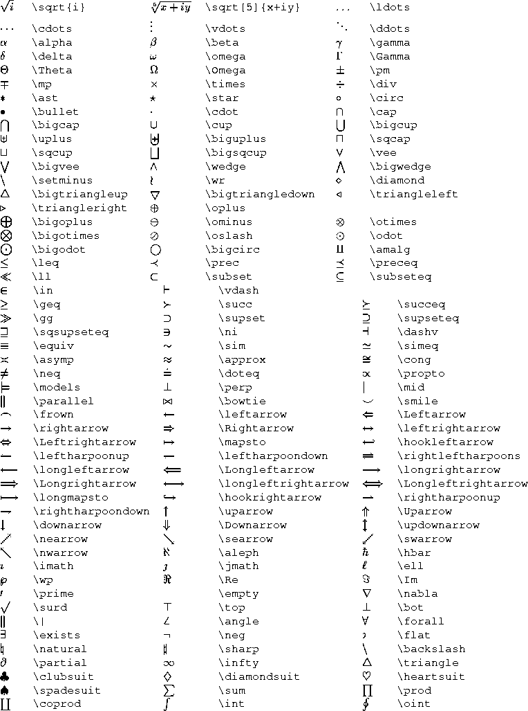
Special characters
Greek
Misc.
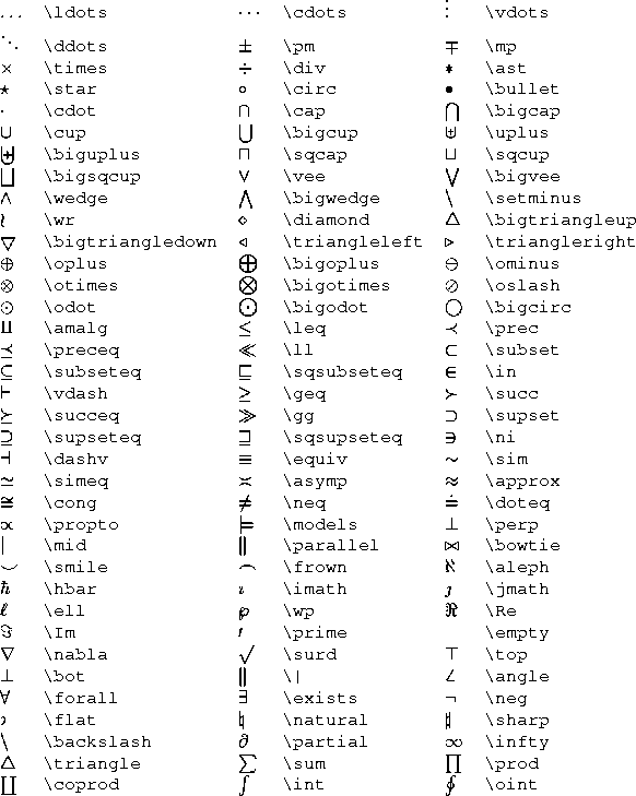
Arrows
![]()
Calligraphic
These characters are available if you use the \cal control sequence.
${\cal A B C D E F G H I J K L M N O P Q R S T U V W X Y Z}$
gives

Character modifiers

Note that the wide versions of hat and tilde cannot produce very wide alternatives. The `\not' operator hasn't properly cut the following letter. The Fine Tuning section describes how to adjust this.
If you want to place one character above another, you can use \stackrel, which prints its first argument in small type immediately above the second
$ a \stackrel{def}{=} b + c $
gives

See the Macros section for how to stack characters using atop.
Common functions
In a maths environment, LaTeX assumes that variables will have single-character names. Function names require special treatment. The advantage of using the following control sequences for common functions is that the text will not be put in math italic and subscripts/superscripts will be made into limits where appropriate.

Subscripts and superscripts
These are introduced by the `^' and `_' characters. Depending on the base character and the current style, the sub- or superscripts may go to the right of or directly above/below the main character. With letters it goes to the right.
$F_2^3$
Overlining, underlining and bold characters
${\underline{one}} {\overline{two}}$
This is not a useful facility if it's used more than once on a line. The lines are produced so that they don't quite overlap the text; lines over or under different words won't in general be at the same height.
\mathbf{} can be used to create bold characters. $\mathbf{F}_2^3$.
To be able to reproduce bold greek characters you can try the amsbsy package then use something like $\pmb{\Gamma}$. Alternatively, you can use the following idea
\usepackage{amsbsy} % This loads amstext too
\begin{document}
$\omega + \boldsymbol{\omega}$

% Use the following if whole expressions need to be in bold
{\boldmath $\omega $}
\end{document}
Roots
$\sqrt{4} + \sqrt[3]{x + y}$
Fractions
Three constructions for putting expressions above others are
- frac: $\frac{1}{(x + 3)}$
- choose: ${n + 1 \choose 3}$
- atop: ${x \atop y}$
These constructions can be used with ones described earlier. E.g.,
\[ \sum_{-1\le i \le 1 \atop 0 < j < \infty} f(i,j)\]
Delimeters

This table shows the standard sizes. To get bigger sizes, use these prefices

For example,
$\Biggl\{2\Bigl(x(3+y)\Bigr)\Biggr\}$
If you're not using the default text size these commands might not work correctly. In that case try the exscale package.
It's preferable to let LaTeX choose the delimiter size for you by using \left and \right. These will produce delimiters just big enough for the formulae inbetween.
$\left( frac{(x+iy)}{\{\int x\}} \right)$
The left and right delimiters needn't be the same type. It's sometimes useful to make one of them invisible
\[ z = \left\{
              \begin{array}{ll}
                   1 & (x>0)\\
                   0 & (x<0)
              \end{array}
       \right.
\]
Over- and underbracing works too.
$\overbrace{\alpha \ldots \omega}^{\mbox{greek}}
\underbrace{a \ldots z}_{\mbox{english}}$
The use of \mbox stops the text appearing in math italic.
Numbering and labelling
Numbering happening automatically when you display equations. If you don't want an equation numbered, use \nonumber beside the equation. Equation numbers appear to the right of the maths by default. To make them appear on the left use the leqno class option (i.e., use \documentclass[leqno,....]{....}).
Use \label{} to label an equation (or figure, section etc) in order to reference from elsewhere.
\begin{equation}
W_{\bf S}(t,\omega) = \int\limits_{-\infty}^{\infty} {
  {\cal R}_{\bf S}(t,\tau) e^{-j\omega\tau} \,d \tau }
\label{LABELLING}
\end{equation}
Now the following text
refers back to equation \ref{LABELLING}
refers back to equation <number> by number, and
refers back to the equation on page \pageref{LABELLING}
refers back to the equation on page NN.
A file will have to be LaTeX'ed twice before the references, both forwards and backwards, will be correctly produced.
Matrices
The array environment is like LaTeX's tabular environment except that each element is in math mode. The default font style used is text style but you can override this by using \displaystyle.
\begin{math}
\begin{array}{clrr} %
      a+b+c & uv & x-y & 27 \\
       x+y  & w  & +z  & 363
\end{array}
\end{math}
The rows are arranged so that their centres are aligned. You can align their tops or bottoms instead by using a further argument when you create the array.
\begin{array}{clrr}[t]
would produce top-aligned lines, and `[b]' would produce bottom-aligned ones. The Delimiters section of this document shows how to bracket matrices.
TeX has a few maths facilities not mentioned in the LaTeX book. The following TeX construction might be useful.
\begin{math}
\bordermatrix{&a_1&a_2&...&a_n\cr
          b_1 & 1.2  & 3.3  & 5.1  & 2.8  \cr
          c_1 & 4.7  & 7.8  & 2.4  & 1.9  \cr
          ... & ...  & ...  & ...  & ...  \cr
          z_1 & 8.0  & 9.9  & 0.9  & 9.99  \cr}
\end{math}
Macros
These aid readability, save on repetitive typing and offer ways of producing stylistic variations on standard LaTeX formats.
\def\bydefn{\stackrel{def}{=}}
\def\convf{\hbox{\space \raise-2mm\hbox{$\textstyle
    \bigotimes \atop \scriptstyle \omega$} \space}}
offer the "new" and shorter commands $\bydefn$ and $\convf$.
Packages
The following packages may be of help :
- easybmat - easy block matrices
- easyeqn - easy equations.
- easymat - easy matrices
- easytable - easy tables
- easyvector - easy vectors
- delarray - nested arrays
- theorem - gives more choice in theorem layout
- subeqnarray - Renumbering of sub-arrays in math-mode
- subeqn - Different numbering sub-arrays
Fine tuning
It's generally a good idea to keep punctuation outside math mode; LaTeX's normal handling of spacing around punctuation is suspended during maths. Sometimes you might want to adjust the spacing in a formula (e.g., you might want to add space before dx). Use these symbols :

In an eqnarray environment you may want to break a long line. You can do this by putting
y & = & a + b \nonumber \\
  &   & + k
but the spacing around the `+' on the 2nd line is wrong because LaTeX thinks it's a unary operator. You can fool LaTeX into treating it as a binary operator by inserting a hidden character.
y & = & a + b \nonumber \\
  &   & \mbox{} + k
You can use the \lefteqn construction to format long expressions so that continuation lines are differently indented.
\begin{eqnarray}
\lefteqn{x+ iy=}\\
& & a + b + c + d + e + f + g + h + i + j + k +\nonumber\\
& & l + m \nonumber
\end{eqnarray}
If you want more vertical spacing around a line you can create an invisible vertical "struct" in LaTeX. \rule[-.3cm]{0cm}{1cm} creates a box of width 0, height 1cm which starts .3cm below the usual line base. By adjusting these values you should be able to create as much extra space below/above the maths as you like.'
Fonts
Font Sizes
These are the available sizes.

If, for example, you want to use the smallest size, do
{\tiny ... }
If Huge isn't big enough for you, you can scale a postscript font up using the commands designed for graphics, \resizebox{!}{5cm}{BIG}.
Font Types
Independent of size, these font types are at your disposal : \textrm (roman), textit(italic), \textsc (SMALL CAPS), \emph (emphasis, but note that if you use emph within emphasized text, you will get roman text), \textsl (slanting), \texttt (teletype), \textbf (boldface), \textsf (sans serif). As long as there's no conflict, these commands can be combined so that, for instance, this is bold sans serif can be produced by \textsf{\textbf{this is bold sans serif}}.
Font attributes
Every text font in LaTeX has five attributes:
- encoding: This specifies the order that characters appear in the font. The most common values for the font encoding is OT1.
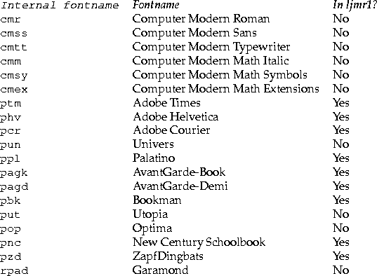
- family: The name for a collection of fonts, usually grouped under a common name by the font foundry. For example, `Adobe Times' and Knuth's `Computer Modern Roman' are font families. There are far too many font families to list them all, but some common ones are:
- series: How heavy or expanded a font is. For example, `medium weight', `narrow' and `bold extended' are all series. The most common values for the font series are:
| m | Medium |
| b | Bold |
| bx | Bold extended |
| sb | Semi-bold |
| c | Condensed |
- shape: The form of the letters within a font family. For example, `italic', `oblique' and `upright' are all font shapes. The most common values for the font shape are:
| n | Normal (that is "upright" or "roman") |
| it | Italic |
| sl | Slanted (or "oblique") |
| sc | Caps and small caps |
- size: The design size of the font, for example `10pt'.
These five parameters specify every LaTeX font, for example:

Selection commands
There are commands to set attributes one at a time: Command Attribute Value in article class, 10pt
| Command | Attribute | Value in article class, 10pt |
|---|---|---|
| \textrm{...} or \rmfamily | family | cmr |
| \textsf{...} or \sffamily | family | cmss |
| \texttt{...} or \ttfamily | family | cmtt |
| \textmd{...} or \mdseries | series | m |
| \textbf{...} or \bfseries | series | bx |
| \textup{...} or \upshape | shape | n |
| \textit{...} or \itshape | shape | it |
| \textsl{...} or \slshape | shape | sl |
| \textsc{...} or \scshape | shape | sc |
| \tiny | size | 5pt |
| \scriptsize | size | 7pt |
| \footnotesize | size | 8pt |
| \small | size | 9pt |
| \normalsize | size | 10pt |
| \large | size | 12pt |
| \Large | size | 14.4pt |
| \LARGE | size | 17.28pt |
| \huge | size | 20.74pt |
| \HUGE | size | 24.88pt |
The low-level commands used to change font attributes are as follows.
- \fontencoding{encoding}
- \fontfamily{family}
- \fontseries{series}
- \fontshape{shape}
- \fontsize{size}
Each of these commands sets one of the font attributes; \fontsize also sets \baselineskip. The actual font in use is not altered by these commands, but the current attributes are used to determine which font to use after the next \selectfont command.
\selectfont selects a text font, based on the current values of the font attributes. There must be a \selectfont command immediately after any settings of the font parameters by (some of) the five \font<parameter> commands, before any following text. For example, it is legal to say:
\fontfamily{ptm}\fontseries{b}\selectfont Some text.
to select bold Times Roman, but it is not legal to say:
\fontfamily{ptm} Some \fontseries{b}\selectfont text.

\usefont{encoding}{family}{series}{shape}
is short hand for the equivalent \font... commands followed by\selectfont.
Examples
A Thesis
To illustrate aspects of writing a LaTeX document and using Emacs to do so we will here show how a thesis could be setup. As mentioned earlier it is convenient to divide larger documents in eg. chapters and then insert the files containing the various chapters using the \include command. Typically you would want your thesis to include :
- a title page
- a preface
- a table of contents (TOC)
- a list of figures (LOF)
- a list of tables (LOT)
- a body containing the actual thesis
- a reference list (bibliography)
- an appendix
From your main-document you can load/insert the elements containing the text and add other commands, eg. numbering methods, header setup, etc. Here is a sample main-document :
In this example we have used the "book"-style to allow chapters. Various packages are loaded. The Natural Sciences bibliography package natbib is among the most complete (see natbib.dvi for more info). There is a redefinition of the header, taken from the fancyhdr.dvi document. Then the definition of the titlepage variables and a list of files to include. This command does not actually include the files (this is done using the \include further down), but tells latex which of these should actually be included (instead of commenting the include-statements). Within the "document" environment we load the acronym definitions, display the titlepage, define pagenumbering to roman, insert preface, make TOC, LOF and LOT (with additional commands to include these in the TOC), change to arabic page numbering, insert the chapters, make the bibliography and start the appendix (inserting two appendix-parts). After successful compilation, the dvi-document can be view :
Compilation consists of :
> latex thesis
> latex thesis
> bibtex thesis
> latex thesis
Note that the bibliography list is made during compilation. The bibliography mybib.bib can be a general list of references which can be used in many different documents. The \citecommands (actually \citet and \citep as defined in natbib.dvi) are used to refer to a reference in the bib-list and the bib-list entry for that reference is then automatically inserted in the bibliography of the current document. There are various bibliography styles (what the bibliography should look like in your document), here we've used the astron.bst style.
To edit the bib-list, eg. mybib.bib you can load it into emacs, which will automatically recognize it as such (.bib) and start the bibtex-mode.
Environment variables
There are a few LaTeX specific UNIX environment variables that can be set to customize LaTeX for you. You can for instance set which LaTeX version to use as default by setting :
setenv LATEXIS latex2e
Your personal .sty, .bib and .bst files should be placed in an appropriate directory under your account and the path specified to the following UNIX environment variables, respectively :
setenv TEXINPUTS .:~/tex/inputs:
setenv BIBINPUTS .:~/tex/bibinputs:
setenv BSTINPUTS .:~/tex/inputs:
LaTeX will then also look for files in those directories in addition to the standard distribution directories.