Confidence Curves for Dummies

We are actually 95 percent confident that 95 percent of readers of our FocuStat Blog Posts are not really "dummies". At any rate we aim here at giving you the basics of confidence curves and confidence distributions, explaining what they are, what they tend to look like, how they can be interpreted, used, and combined, though largely without the technical details.

We start with a simple example and then jump a bit from theme to theme, partly by illustrations where most of the math has been snipped away.

A start example

Here's a simple example. You observe the data points 4.09, 6.37, 6.87, 7.86, 8.28, 13.13 from a normal distribution and wish to assess the underlying spread parameter, the famous standard deviation $\sigma$. We'll now introduce you to as many as two (2) curves: the confidence curve ${\rm cc}(\sigma)$ and the confidence distribution $C(\sigma)$. They're close cousins, actually, and it's not the case that both curves need to be displayed for each new statistical application.

The confidence curve shown in Figure A sums up what can be told from the data about that particular parameter (in companionship with the statistical model at work). It has candidate values $\sigma$ on the horizontal axis and level of confidence on the vertical axis. One of these parameter values is the true one, the one "behind the data". Even a statistician can't tease out which $\sigma$ is the true one, but we can estimate it (with better precision, if given more data), and can also sort the likely ones from the less likely ones. The ${\rm cc}(\sigma)$ is a graphical mini-summary of various calculations relating to such efforts:

• it points to the point estimate (naturally), here 3.226 (which we call the median confidence estimate);
• we may read off e.g. a 90 percent confidence interval of likely values for $\sigma$, here $[2.023, 6.286]$, see the red horizontal dotted line, and the corresponding two blue marks on the $\sigma$ axis;
• intervals for any other level of confidence may be read off too; and
• we see the clear asymmetry in how confidence is distributed.

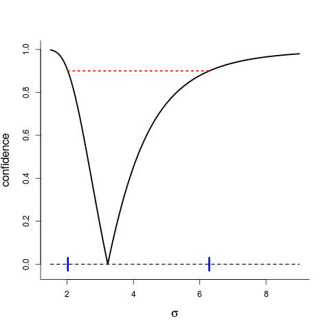
_{Figure A: confidence curve ${\rm cc}(\sigma)$ for the $\sigma$ parameter, the unknown standard deviation of the distribution behind the data. We read off the point estimate at 3.226 (it's the median confidence point estimate), read off confidence intervals, like $[2.023, 6.286]$ at level 90 percent, etc.}

In many other cases the confidence curve is symmetric, or closer to symmetric, but here the distribution of the statistic informing us about the size of $\sigma$ has a skewed disribution (a bit away from the ubiqitous Gaussian or normal distributions).

A sister version of the confidence curve ${\rm cc}(\sigma)$ is the cumulative distribution function $C(\sigma)$, shown in Figure B. It's often called the CD, the confidence distribution. It starts at level 0 far to the left and climbs up to level 1 far to the right. It passes the magical midpoint 0.50 at the median confidence point estimate 3.226. At position 2.023 the CD is equal to 0.05, which means 5 percent confidence in everything to the left and 95 percent in everything to the right. Similarly, at position 6.286 the CD is equal to 0.95, with 5 percent confidence in everything to the right of that value, etc. So there's 90 percent confidence in the interval of all values from C-inverse of 0.05 to C-inverse of 0.95, that is, 2.023 to 6.286, corresponding to what we read off from the ${\rm cc}(\sigma)$ curve. 

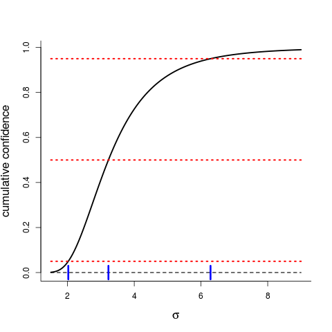
_{Figure B: confidence distribution function $C(\sigma)$ for $\sigma$, for the same situation and the same data as for Figure A. The 90 percent confidence interval is read off from when the cumulative crosses 0.05 (at 2.023) to when it crosses 0.95 (at 6.286). It crosses the 0.50 level at the median confidence estimate 3.226}

We can construct $C(\sigma)$ from ${\rm cc}(\sigma)$ and vice versa. We prefer the cc over the CD in many regular cases, but the CD is sometimes better when it comes to emphasing irregularities, like when a single borderline point has a positive probability (Figure C below is a case in point).

A note here, for added understanding of what goes on, is that with more data, precision improves, leading to slimmer confidence intervals and tighter confidence curves. Any crucial statistical parameter $\gamma$ dreams of good-quality data flowing from well-designed experiments related directly or at least indirectly to precisely that parameter. Then good statisticians will model away, perform magic at the required level, and land a strong, informative, slim, steep ${\rm cc}(\gamma)$.

It's an inferential summary

So the confidence curve (and its cumulative sister, the confidence distribution) is an inferential summary. It presents the main result of a statistical analysis, for each of the parameters we might be interested in, and constitutes a foundation from which the user and the public can draw real-world conclusions to quantitative problems (and authorities can start making decisions).

All quantitative researchers and an increasing part of the population at large are familiar with point estimates, confidence intervals, and p-values. A point estimate is an intelligent guess of the correct value of the parameter in question; a confidence interval gives a set of likely values; a p-value allows the user to conclude a hypothesis test. The confidence curve offers these things, and more. 

Going back to the (very) simple dataset above, suppose there is interest in testing whether $\sigma\le 2.00$ (imagine, if your imagination needs a pedagogical momentum for such things, that 2.00 is the magical industry standard for such measurements, and that the new measurements relate to a new expensive machine). Should we accept the $H_0\colon \sigma\le 2.00$ hypothesis, or should we reject it (which is the statistical parlance around hypothesis testing)?

Well, we read off $p=C(2.00)=0.045$ from the CD, and are not particularly confident in the null hypothesis. This is the p-value! So standard practice here would be to cast away $H_0$, in that the data indicate it's wrong; there is considerably more confidence in the alternative $\sigma>2.00$ being right.

CDs, p-values, and distance-from-null parameters

We have access to birthweight data for a cohort of children born at the Rikshospitalet in Oslo in the 2001-2008 period. It's pretty clear that boys are bigger than girls, on average; the means are actually 3.669 kg for $n_b=548$ boys and 3.493 kg for $n_g=480$ girls. But is the statistical spread for boys also bigger than for the girls? Let's check the ratio of standard deviations

\(\rho=\sigma_b/\sigma_g.\)

Let's also make it part of our assumptions about the world that $\sigma_b$ should not really be smaller than $\sigma_g$, since there are so many biological traits which are more variable for boys than for girls. So our statistical task is to estimate $\rho$ and assess its uncertainty, and our statistical summary answer is the CD of Figure C, the $C(\rho)$.

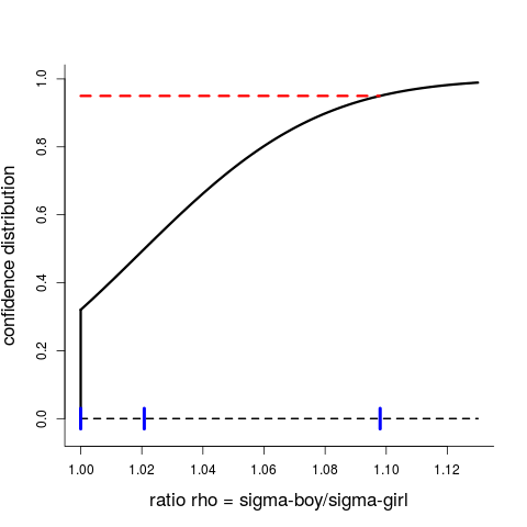
_{Figure C: CD for $\rho=\sigma_b/\sigma_g$, starting at 1.00. We read off the p-value $C(1)=0.320$ for testing the null hypothesis that the two standard deviations are the same; the median confidence estimate 1.021 where the CD crosses 0.50; and the 95 percent interval is from 1.000 to 1.098.}

Estimates of the standard deviations are 0.574 and 0.561 and hence pretty close, which is why the CD is pretty much concentrated on $[1.00,1.12]$, i.e. close to 1. The CD here starts off with a notable point-mass at the left end point, namely $C(1)=0.320$, which is also the p-value for the test of the natural null hypothesis that there is no difference between the two populations regarding spread. Also, the median confidence estimate is found to be 1.021, and the 95 percent interval of confidence is $[1.000,1.098]$, see the blue marks on the horizontal axis.

The more general point to convey here is that far too often statistical testing is reported on in too crude terms; a yes-or-no answer is provided after a hopefully clever testing of the relevant $H_0$ has been carried out, perhaps having used a 0.05 rule of significance. It's a bit more informative to quote also the p-value (like the very non-significant 0.320 for the situation of Figure C). We advocate doing more, via the CDs:

• put up a decent parameter, which signals the "distance to the null", the degree to which the $H_0$ is not holding, in a meaningful and context-driven way; and
• construct a CD for that parameter.

In the boys-and-girls example, telling people that "we tested equality of the two standard deviations, and did not reject that null hypothesis" is less interesting and less informative than giving the full CD for the ratio.

Confident Confidence Curves as standard output in regression models

To make our next point, we've analysed a certain dataset pertaining to $n=189$ mothers and their newborns, where the binary outcome is whether the child is small (less than 2500 g) or not, and the point is to see how the probability

\(p(x_1,x_2,x_3,x_4) = {\rm Pr}({\rm small\ child}\,|\,x_1,x_2,x_3,x_4) = {\exp(\beta_0+\beta_1x_1+\beta_2x_2+\beta_3x_3+\beta_4x_4) \over 1 + \exp(\beta_0+\beta_1x_1+\beta_2x_2+\beta_3x_3+\beta_4x_4)}\)

is influenced by certain covariates. For this analysis these are

• $x_1$, mother's age;
• $x_2$, mother's weight, prior to pregnancy;
• $x_3$, which is 0 for nonsmokers and 1 for smokers;
• $x_4$, which is 0 for white and 1 for non-white.

In order for the logistic regression coefficients $\beta_1,\beta_2,\beta_3,\beta_4$ to be compared usefully on the same statistical footing, we normalise the four covariates by dividing by their standard deviations. Using maximum likelihood theory, both for obtaining the estimates and assessing their distributions, leads with a few more efforts to the four confidence curves ${\rm cc}_j(\beta_j)$ shown in Figure D.

_{Figure D: confidence curves for the regression coefficients $\beta_1,\beta_2,\beta_3,\beta_4$ in the study of how four mother covariates influence the probability that the newborn child will have low birthweight, smaller than 2500 g. The two green dashed curves to the left are for weight and age, and these are in the straight statistical nonsignificant vicinity of zero. The two full curves on the right, one black and one red, are however significantly distanced from zero. So being a smoker and/or being non-white significantly increases the chances of your child being small. The data are from Hosmer and Lemeshow (1989), part of a larger study at Baystate Medical Center, Springfield, Massachusetts; see Claeskens and Hjort (2008) for further analyses.}

Now consider the vertical blue null line, positioned at $\beta=0$. The reading is that

• if the null line is inside the natural statistical grip of the ${\rm cc}_j(\beta_j)$, as with the two green curves a bit to the left, then the coefficients are not significant, and the associated covariates do not significantly influence the probability;
• if the ${\rm cc}_j(\beta_j)$ is clearly a distance away from the null line, as with the black curve (for smoking) and the red curve (for non-white), then these factors are significantly present. 

We invite such Confident Confidence Curves(™) to become part of your standard output when running, analysing, interpreting your regressions. These help you do the traditional sorting of covariates into "significant" and "nonsignificant" categories, but also to see which might be more or much more important than others, and to judge the precision of the coefficients. For this illustration we also discover the somewhat surprising thing that being a smoker and being non-white exert virtually identical influences on the small baby probability.

Such regression analyses should typically be followed by careful estimation and assessment of context-driven focus parameters, aspects of the situation which matter. If Mrs. Jones is pregnant (and she apparently is, see Cunen and Hjort, 2020a), she would care about $p_{\rm jones}$, her own probability, a function of the five parameters in the bigger model, and then there is methodology to provide a ${\rm cc}(p_{\rm jones})$ for that parameter too.

The world's first novel: when did Author B take over for Author A?

Full of adventures, battles and love stories, the chivalry romance Tirant lo Blanch is a masterpiece of medieval literature (written in Catalan, in the 1460ies, 150 years before Don Quijote). It contains also a certain statistical mystery: its primary author Joanot Martorell died before the story was completed, so from which chapter onwards did his friend Martí Joan de Galba take over?

So we read the book's 487 chapters, with the rapt attention demanded of us as readers and statisticians; properly catalogued the Catalan word length distributions, chapter by chapter by chapter; diligently modelled the full process via nine-dimensional Gaussian distributions; put everything into a somewhat elaborate change-point model of our own making; and landed at Figure E, the confidence curve for the chapter at which the transition from Author One to Author Two took place. Our point estimate is $\hat\tau=371$, with confidence sets at different confidence levels to be read off from the curve. Intriguingly, the apparatus detects a second lower-probability possibility for the Author Shift Point, at chapter 342.

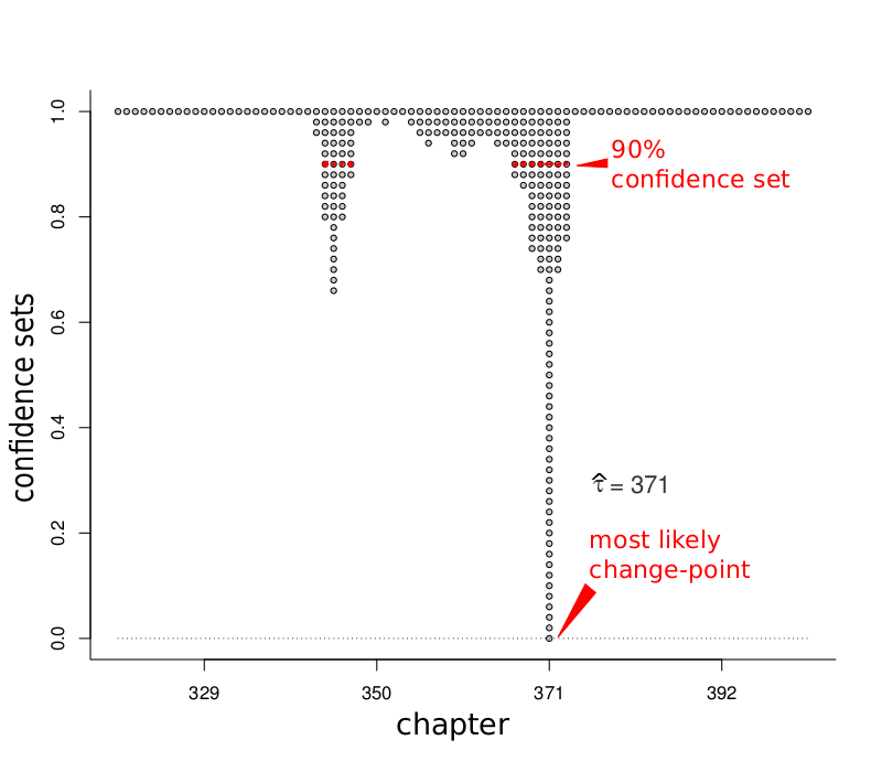
_{Figure E: zooming in on the range of chapters where statistical sightings of change-point action take place, regarding the mechanics of word-length distributions across chapters, the figure gives ${\rm cc}(\tau)$, the confidence curve for the change-point chapter $\tau$, where Author Two takes over for Author One.}

Where are the snows of yesteryear?

Have a look at Figure F, which has the statistical power to scare some of us, as it carries the deep-climatic message that the number of skiing days at Bjørnholt (an hour's cross-country skiing into Nordmarka, close to Oslo) might be in decline.

_{Figure F: the number of skiing days per year, recorded 102 times in the period from 1897 to 2015, at lovely Bjørnholt a skiing distance from the University of Oslo Blindern campus, with a skiing day defined as there being at least 25 cm snow on the ground. The red dashed curve is the signal, the estimated quadratic trend; read Heger.}

We've fitted a simple regression model with quadratic trend,

\(y_i = \beta_0 + \beta_1 x_i + \beta_2 x_i^2 + \varepsilon_i, \)

for $i=1,\ldots,n$, with $x_i$ the calendar year in question and $y_i$ the number of skiing days. We think about the quadratic $\beta_0+\beta_1 x+\beta_2 x^2$ as the signal and the so-called error zero-mean terms $\varepsilon_i$ as the noise. For the present purposes we do not go into deeper modelling and view these $\varepsilon_i$ as independent with the same distribution, where their standard deviation $\sigma$ has a role to play.

Lucikly the $\sigma$ is relatively high, estimated at $\hat\sigma=37.04$, which means there'll be a fair amount of up-and-down winters around the signal (the red dashed curve in Figure E). Thus there can be a few bad winters before we're blessed by better winters again (translate this to "more skiing").

Figure G relates to one of several hard questions Norwegians can ask about the future, the climate, and everything: will the signal itself, the expected number of skiing days, ever come all the way down to certain painful lower levels, like $d_0=45$ skiing days? The figure gives us ${\rm cc}(x_0)$, for the unknown future calendar year $x_0$, where

\({\rm E}(y\,|\,x_0) = \beta_0 + \beta_1 x_0 + \beta_2 x_0^2 = 45.\)

This is actually a harder task than the traditional ones dealt with in regression models, since the solution to this equation yields $x_0$ in terms of three unknown parameters, giving $\hat x_0$ a somewhat complicated distribution, etc. Interestingly and perhaps comfortingly, the ${\rm cc}(x_0)$ is not only rather skewed to the long right, but the curve stops climbing, reaching a finite asymptote below 0.70.

Even though our data and model lead to the point estimate $\hat x_0=2066$, the bad year where we can only ski 45 days at Bjørnholt, there's a fair chance that it will never happen. The 80 percent confidence interval, for this tricky future parameter, stretches from 2040 to, well, infinity. Of course there are a few other key assumptions in such calculations, incuding the one about time-stationarity, that both the signal and the noise in the key modelling equation above will behave more or less as they have over the past hundred years or so.

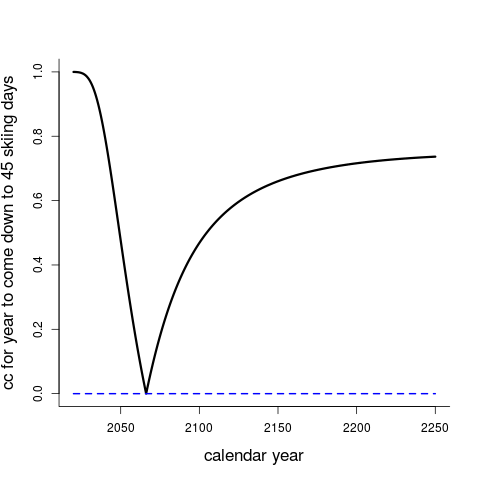
_{Figure G: the confidence curve ${\rm cc}(x_0)$ for the future calendar year, which may or may not actually take place, where the mean level $\beta_0+\beta_1 x_0+\beta_2 x_0^2$ for the number of skiing days reaches all the way down to 45 days.} 

Combining information across diverse sources

Suppose we need to know something about a certain parameter, like the corona pandemic reproduction number $R_0$ for the society we live in, perhaps influenced by various decisions and by yet other partly unknown quantities. There would typically be several sources of information, and these again might be of rather different sort, regarding data quality, precision, direct or indirect relevance to the most crucial questions, etc.

The confidence curves can play vital roles in such games, sometimes called meta-analysis. The picture to have in mind is roughly as follows. We're interested in a certain focus parameter, say $\phi$, which for the March-April-May-June 2020 situation alluded to might be the $R_0$, say for Norway. In a proper meta-setup, this $\phi$ is a function of other parameters, say $\theta_1,\ldots,\theta_k$, with $\theta_j$ associated with information from source $j$. In addition to understanding well enough how well these sources work, leading to a little string of ${\rm cc}_j(\theta_j)$, we wish to do "fusion", fuse together the different ${\rm cc}_j(\theta_j)$ to arrive at the most relevant and most precise conclusions.

In Cunen and Hjort (2020b) we have attempted to identify and formalise three natural steps for statistical encounters of this type. The II-CC-FF apparatus has the three steps

• the II, Independent Inspection, where each information source is analysed, whether from raw data or via summary analyses in other people's studies, landing in the relevant confidence curves ${\rm cc}_j(\theta_j)$ for these separate components; 
• the CC, Confidence Conversion, involving the statistical translation of confidence curves to log-likelihood contributions;
• the FF, Focused Fusion, the final fusion step, leading to the ${\rm cc}_{\rm fusion}(\phi)$, the best statistical knowledge we can have concerning $\phi$, based on comibining the different sources of information. 

Readers wishing to see more details, regading the concepts, the theory, and applications, need to go to the, well, sources, i.e. our journal paper. But here is a moderately simple illustration of what goes on. In six different studies one analyses and compares a new lidocaine type drug with a placebo, and for the present illustration agree that this amounts to analysing the same statistical effect parameter $\gamma$ for six different setups. This gives rise to the six thinner lines ${\rm cc}_j(\gamma)$ in Figure H, corresponding to the II step above.

Then there are as many as two additional curves in the diagram, both representing statistical fusion across the six studies, say ${\rm cc}_{\rm black}(\gamma)$ (black, full) and ${\rm cc}_{\rm red}(\gamma)$ (red, dashed). The first is the guaranteed optimal confidence curve, utilising all raw data in the proper meta-model. The second has bypassed the raw data, and is utilising information only from the ${\rm cc}_j(\gamma)$ curves, via our II- and FF-machinery.

We see that the II-CC-FF apparatus, using essentially summary information (but nothing else) from the six studies, is able to match the more elaborate all-raw-data method. This is of course promising in that the proverbial modern statistician – carrying out the proverbially modern complicated challenging important tasks of combining perhaps very diverse sources of information, with the government tapping their fingers in eager anticipation – typically does not have access to all the raw data and their details. So this is (or might be) the statistics of clever summary statistics of summary statistics.

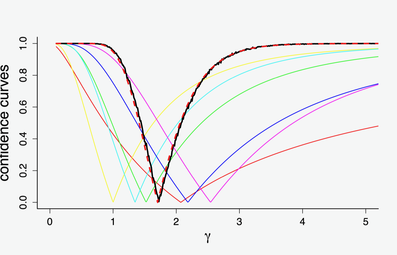
_{Figure H: six different lidocaine studies give rise to the six confidence curves ${\rm cc}_j(\gamma)$, shown as thinner lines. Then there are two fatter lines in the middle, both representing statistical fusion over the six sourcess. The full black  curve is the genuinely optimal confidence curve, utilising the raw data for all six sources, in the proper meta-model. The red dashed curve is the result of our II-CC-FF procedure, which only uses summary information from the individual studies.}

In many other applications things are more complicated, also since it famously happens that not all sources of information agree so well. Hence a good statistical meta-summary should take such a degree of partial disagreement into account as well, and perhaps present it as part of the current state of knowledge. The II-CC-FF can do that as well.

A few notes & footnotes

The active use of confidence curves and confidence distributions should discourage the automatic use of statistical methods and algorithms, and rather encourage critical thinking and the use of different sources of information to reach better overall conclusions and decisions. The confidence curve promotes transparency: given the same data and assumptions, different users should arrive at the same confidence curve, but might nonetheless reach different real-world conclusions in the end. 

Here's a list of concluding comments.

A. At the basic level the confidence curve is simply a plot of nested confidence intervals at all levels, from 0 to 100 percent. The plot conveys a lot of information quickly and is easy to understand. Some users will interpret this as a distribution of likely values, after seeing the data; it is indeed the canonical frequentist cousin of the Bayesian's posterior density (but there is no prior camel to swallow).

B. Confidence distributions and confidence curves have a somewhat long and partly complicated history, also because some proponents might have been overselling their uses and misunderstood some of their limitations. These controversies, coupled with too short lists of convincing applications, have contributed to the sociological fact that $C(\gamma)$ and ${\rm cc}(\gamma)$ have not yet reached Mainstream Statistics (but we're working on it).

The ambition level is high – Brad Efron (who is 50 percent of the statisticians of the world upon whom has been bestowed an honoris causa doctoral degree from the University of Oslo) more or less says that this is The Holy Grail of Statistics, having a coherent well-working well-understood way of creating posterior distributions for focus parameters without priors. And we, as in Schweder and Hjort and C. Cunen and M. Xie and R. Liu and J. Hannig and X. Meng and R. Gong and R. Martin and a significant wave of BFFers (there's a sequence of conferences on Bayesian, Frequentist, Fiducial themes), more or less say that the CDs and the ccs are, well, it. See Schweder and Hjort (2016, Ch. 6) for a discussion of the history, from R.A. Fisher's fiducial distributions of 1930 and onwards.

C. This blog post is perhaps not "for dummies", after all, but we've kept it low on the math and the technical details. Let us briefly point to two good recipes, though. The first is based on a traditional normal approximation: if $\hat\gamma$ is a good estimator of the parameter $\gamma$, and its distribution is approximately a ${\rm N}(\gamma,\hat\tau^2)$, then

\(C(\gamma) = \Phi\Bigl({\gamma-\hat\gamma\over \hat\tau}\Bigr)\)

can be used, with $\Phi$ the standard normal cumulative distribution function. Also, the associated (approximate) confidence curve is

\({{\rm cc}}(\gamma) =|1-2\,C(\gamma)| =\Big| 1-2\,\Phi\Bigl({\gamma-\hat\gamma\over \hat\tau}\Bigr) \Big|.\)

In typical cases, the $\hat\tau$ here goes down in size inversely proportional to $\sqrt{n}$, with $n$ being the sample size for the data that led to the computation of $\hat\gamma$ in the first place. Incidentally, this approximation to a ${\rm cc}(\gamma)$ is closely related to what one learns in school, that an approximate 95 percent confidence interval is $\hat\gamma\pm1.96\,\hat\tau$, etc. This is also operationally speaking the Bayesian answer, having started with a flat prior for the $\gamma$, though the CD perspective and interpretation are different.

D. A more elaborate but still generic method is as follows, in situations where the focus parameter $\gamma$ is a smooth function $\gamma=g(\theta)$ of the model parameter vector $\theta=(\theta_1,\ldots,\theta_p)$. From the model's log-likelihood function $\ell(\theta)$, form first the profiled log-likelihood function

\(\ell_{\rm prof}(\gamma) =\max\{\ell(\theta)\colon g(\theta)=\gamma\}, \)

and then compute what Schweder and Hjort (2016) call the deviance function,

\(D(\gamma)=2\{\ell_{\rm prof,\max}-\ell_{\rm prof}(\gamma)\}. \)

The confidence curve for $\gamma$, using this recipe, is

\({\rm cc}(\gamma) =\Gamma_1(D(\gamma)) ={{\rm pchisq(devvalues,1)}}, \)

in R language, with $\Gamma_1$ being the chi-squared cumulative with 1 degree of freedom.

E. More widely, each procedure for cranking out a confidence interval, in a given type of situation (which means an apparatus for the type of data and one or more models for these), can be adapted to construct a confidence curve. Various recipes, for many types of models and parameters and going beyond Recipies One and Two above, are constructed and applied in Schweder and Hjort (2016). Some procedures are more clever than others, and the book mentioned also delves into such issues, with performance and comparisons, etc.

F. The nonstandard-looking ${\rm cc}(x_0)$ of Figure G is related to a classic problem in statistical inference, called the Fieller problem, where at least some confidence interval constructions might entail infinite or disjoint segments. We believe our confidence curves provide the most satisfactory solutions.

G. The themes involving and related to confidence curves are very much an active research area, where many issues and problems are not yet worked out to satisfaction and mainstream use. Review articles, with longer discussions and ranges of different applications and problems, include Xie and Singh (2013) and Hjort and Schweder (2018). And welcome to Nils Lid Hjort's Master- and PhD-level course STK 9180, more or less on Confidence, Likelihood, Probability, at the Department of Mathematics, University of Oslo.

Thanks

We are grateful to Tore Schweder and Emil Aas Stoltenberg for helpful discussions and comments.

A few references

Claeskens, G., Hjort, N.L. (2008). Model Selection and Model Averaging. Cambridge Unviersity Press, Cambridge.

Cunen, C., Hermansen, G.H., Hjort, N.L. (2018). Confidence distributions for change-points and regime shifts. Journal of Statistical Planning and Inference vol. 195, 14-34.

Cunen, C., Hjort, N.L. (2017). New statistical methods shed light on medieval literary mystery. FocuStat Blog Post.

Cunen, C., Hjort, N.L. (2020a). Confidence distributions for FIC scores. Submitted for publication.

Cunen, C., Hjort, N.L. (2020b). Combining information across diverse sources: the II-CC-FF paradigm. Scandinavian Journal of Statistics [to appear].

Cunen, C., Hjort, N.L., Nygård, H.M. (2020). Statistical Sightings of Better Angels: analysing the distribution of battle-deaths in interstate conflict over time. Journal of Peace Research, 1-14.

Cunen, C., Hjort, N.L., Schweder, T. (2020). Confidence in confidence distributions! Proceedings of the Royal Society A (Mathematical, Physical and Engineering Sciences) [too appear].

Heger, A. (2007). Jeg og jordkloden. Dagsavisen.

Hjort, N.L., Schweder, T. (2018). Confidence distributions and related themes. General introduction article to a Special Issue of the Journal of Statistical Planning and Inference dedicated to this topic, with eleven articles, and with Hjort and Schweder as guest editors; vol. 195, 1-13.

Hjort, N.L. (2020). Koronakrisen: plutselig ble statistikk allemannseie. Interview in Titan, University of Oslo.

Hosmer, D.W., Lemeshow, S. (1989). Applied Logistic Regression. Wiley, New York.

Schweder, T., Hjort, N.L. (2016). Confidence, Likelihood, Probability: Statistical Inference with Condidence Distributions. Cambridge University Press, Cambridge.

Xie, M.-g., Singh, K. (2013). Confidence distribution, the frequentist distribution estimator of a parameter: a review. International Statistical Review, vol. 81, 3-39. Discussion contributions (by Cox, Efron, Fraser, Parzen, Robert, Schweder and Hjort), 40-79.