Your Mother is Alive with Probability One Half

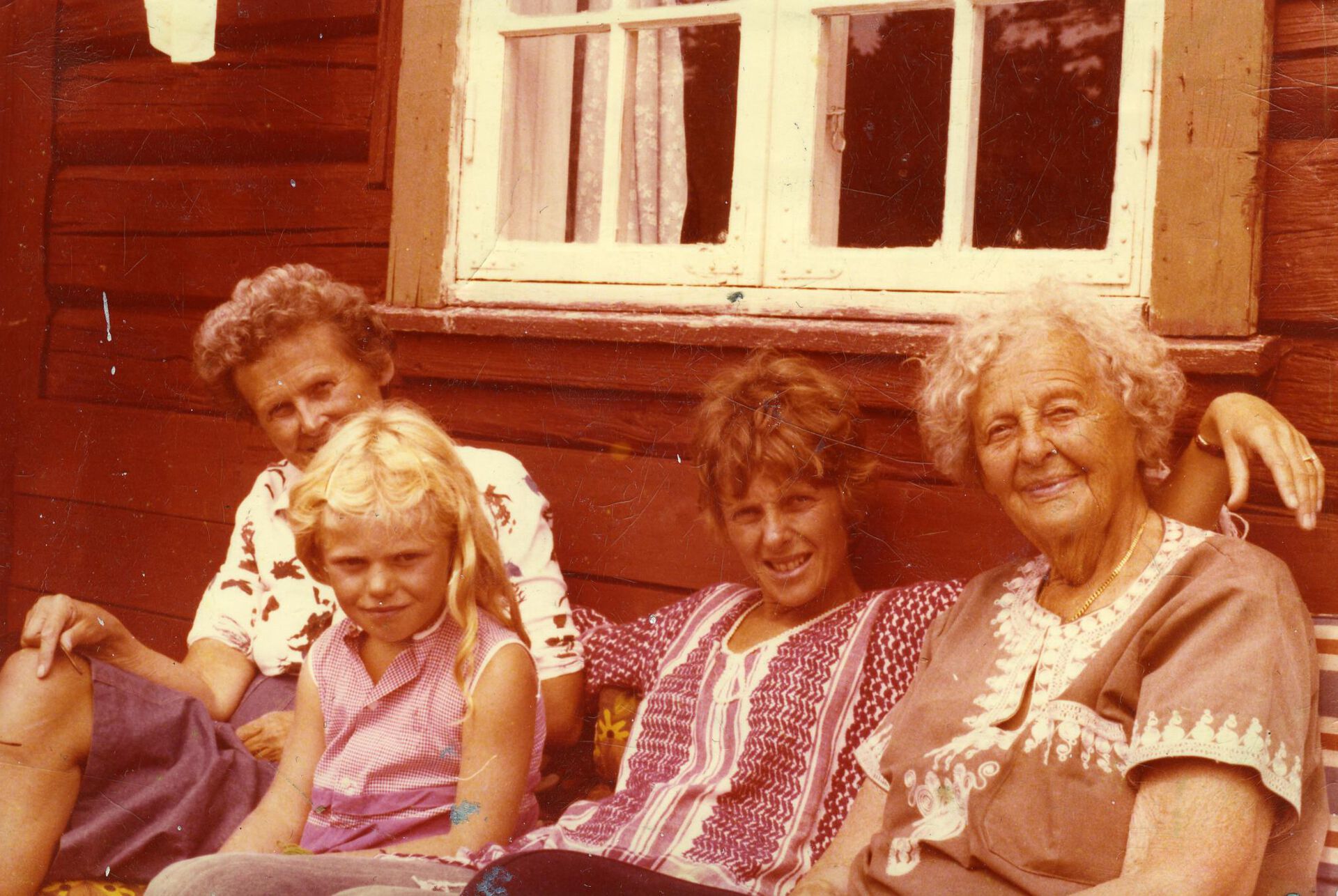
^{Long live daughter, mother, grandmother, great-grandmother. (From the close-kin mark-recapture family archives of Hjort & Heger.)}

Suppose I spend a day interviewing 1000 women on Karl Johans gate, also asking them if their mothers are alive. How many of them will say "yes"? The answer is: about 500 (give or take the binomial variation involved).

Pr(she's alive) = 0.50

There are actually several different sets of assumptions securing this $p=0.50$ answer. Each mother in question is either alive or dead, and this is not a blog post on Schrödinger's mother being both alive and dead – Georgina Bauer Schrödinger, my third great uncle's second cousin twice removed's husband's daughter's husband's brother's wife's first cousin once removed's wife's sister, died in 1921, when Erwin was 34. The probability in question is the statistical one, describing how often the statistician learns "yes, she's alive" when asking the question, to certain strata of the population.

The simplest setup is to suppose (a) that the women I sample have ages $t$ stemming from a density $f_0(t)$, (b) that their mothers' lifelengths stem from a density $f(t)$. The probability that a randomly sampled woman's mother will be alive, using $T_0$ to denote the age of the woman asked and $T$ for her mother's lifelength, is then

\(p = {\rm Pr}(T > T_0) = \int_0^\infty \{1-F(t)\}f_0(t)\,{{\rm d}}t,\)

with $F$ the cumulative of $f$. Under the further condition (c), that the two distributions are actually the same, i.e. that my representative sample on Karl Johans gate, of those alive today, of ages between 0 and 111, say, have the same lifelength prospectives as what their mothers had, when they were born, the answer is seen to be $p={1\over 2}$.

It is also clear that the answer $p=0.50$ remains correct under broad stationarity assumptions, also when $(T_0,T)$, the lifelengths of the daughter and the mother, are modelled as being dependent. We may e.g. view these ages as outcomes of a long sequence of maternal lifespans. As long as $T-T_0$ has a (continuous) distribution symmetric around zero, we have $p=0.50$ again.

Famously, the lifespan distribution isn't entirely stationary, however, and the women (and the men) in most societies keep on getting older and older, in the sense of averages and quantiles, and indeed in the sense of the full statistical distribution $F^*(t\,|\,a)$, for women born in calendar year $a$, getting stochastically larger with time. For some of many indications of this, see e.g. my Exam Project for my model selection course STK 4160 at the University of Oslo, June 2017, with data found via the intriguing databases of www.worldlifeexpectancy.com; further lucid discussion is found in Steven Pinker's Enlightenment Now!, Ch. 5.

In yet other words, the $f$ for your mother's lifelength isn't quite the same as the $f_0$ for your own. It's useful to translate the formula above via hazard rates, so let's write $f_0(t)=h_0(t)\exp\{-H_0(t)\}$ and $f(t)=h(t)\exp\{-H(t)\}$, with hazard rates $h_0$ and $h$ and their cumulatives $H_0$ and $H$. Then probability above may then be written

\(p = \int_0^\infty \exp\{-H(t)\}h_0(t)\exp\{-H_0(t)\}\,{{\rm d}}t.\)

If our mothers lived under conditions with hazard rates $h(t)=ah_0(t)$, a proportionality factor $a$ away from our own, then, provided the sampling of the women I ask is representative, the probability becomes

\(p_a = \int_0^\infty \exp\{-(a+1)H_0(t)\}h_0(t)\,{{\rm d}}t=1/(a+1).\)

Notably, this simple answer depends only on the hazard rate proportionality constant $a$, not the hazard rates themselves. So if only 450 of the 1000 women I sample on Karl Johans gate tell me their mothers are alive, I can estimate $a$ (as 1.22, actually), along with a full confidence curve to assess its precision.

These themes may be pursued further, but then requiring more accurate data and modelling. Writing

\(F(t\,|\,b)=1-\exp\{-H(t\,|\,b)\}\)

for the distribution function for lifelengths $T$, for women born $b$ years ago, a more precise version of the fundamental $p$ formula is actually

\(p = \int_0^\infty \exp\{-H(t\,|\,t)\}h_0(t)\exp\{-H_0(t)\}\,{{\rm d}}t,\)

since the first factor in the integrand needs to be the probability that a woman born $t$ years ago has survived precisely these $t$ years. Such information would presumably be available, at least when broken down to age segment intervals, in the data banks of Statistisk Sentralbyrå, or via data and parametric models used in the life insurance industry. Also to be taken into account, if examining the Pr(your mother is alive) question meticulously, is the implication that your mother has at least survived say 17 years on our planet, and also that she's managed to have a child, motherly aspects making her subtly different from the proverbially randomly sampled woman in our country.

From continuous measurements to age groups

Before coming to the fish I need to comment on one more aspect of relevance, namely that the continuous-scale lifelengths are quite often recorded, and only possible to record, via age intervals. Thus rather than knowing that Mrs Smith lived for 81 years and 4 months and 17 days, one merely knows that she's been sorted into the age window of lifelengths in the 80.00 to 84.99 box. This is even more the case when sampling and investigating age-structured populations, like fish and mammals, where the age cannot be pinned down more accurately than to the year-class. In this terrain there is no $p = \int_0^\infty \{1-F(t)\}f(t)\,{{\rm d}}t={1\over 2}$ formula.

There are indeed discrete-world formulae for $p=P(T > T_0)$, along the lines of

\(p = \sum_j P(T_0=t_j) P(T > t_j) = \sum_j f_j(1-f_0-\cdots-f_j),\)

where $f_j$ is the probability of landing in age box no. $j$, say $(t_j,t_{j+1})$ for interval endpoints $t_0<t_1<\cdots$. A simple illustration is for the geometric distribution, with $f_j=(1-\theta)\theta^j$ for $j=0,1,2,\ldots$, for which one finds $p=\theta/(1+\theta)$. So the simple $p=0.50$ insight is messed up by the intervalisation of lives lived, and also calls for various actuarial fixes and half-corrections, perhaps from the assumption that a lifelength inside an interval ought to be approximately uniformly distributed across that interval, etc. Remarkably, in one of the fishing stories pointed to below, the answer to Pr(your mother is alive) still turns out to be 0.50, even when working with interval data, under some conditions on mortality and birth rates. 

Another general formula, to be used with appropriate care with given data, and perhaps with parametric models for the cumulative hazard rate functions $H_0$ and $H$, is

\(p = \int\prod_{[0,t]}\{1 - {{\rm d}}H(s)\} \prod_{[0,t]}\{1 - {{\rm d}}H_0(s)\}\,{{\rm d}}H_0(t),\)

with the products taken over the relevant age windows. Such formulae, with further modifications, are in principle at work when demographers and statisticians attempt to properly formalise the slightly slippery concepts of "expected lifelength for a girl born in Norway in 2019", etc.; see e.g. the informative article by Borgan and Keilman (2019).

Further extensions of the apparatus above might involve placing Beta process priors on one or both of the cumulative hazard rates, to model and then assess the random $p$ coming out of random sampling of different strata. 

Close-kin mark-recapture

My reasons for taking an interest in the Pr(your mother is alive) questions stem partly from listening to fascinating talks by Hans Julius Skaug, first at the Johan Hjort Symposium and then at the Norwegian Statistical Meeting in Stavanger, both in June 2019, and from reading a few of the associated journal papers. With Mark Bravington and others, Skaug is working out truly wondrous methods for assessing abundance and Spawning Stock Biomass for fish and whale populations. These amount to creative and significant extensions and generalisations of the classical capture-mark-recapture methods from the 1960ies and 1970ies.

One may estimate the total membership $N$ in the Norwegian Statistical Association by noting down $n_1$ and $n_2$, the number of participants at the meetings in Fredrikstad 2017 and Stavanger 2019, respectively, along with $K$, the number of us who attended both meetings. Somebody ought to check out the participants lists for these meetings, but let's suppose the $n_1,n_2,K$ numbers were equal to 69, 81, 42. Then the so-called Lincoln-Peterson estimate is

\(\widehat N=n_1n_2/K=133.\)

There are various refinements and extensions, taking into account the statistical fact of life that there's a subset of Norwegian statisticians who place priority close to zero on attending any of these meetings. Such delicate matters need to be modelled and tended to when forming more robust estimates of abundance and biomass, for statisticians and for fish species, since some strata have very low chance of getting caught in the nets. In particular & indeed, $\widehat N=133$ is seriously underestimating the actual $N$, in this case, precisely because different statisticians have different probabilities of allowing themselves to be statistically netted in that fashion. This is actually just as for the Finnish forest mice Microtus agrestis, who had different appetites for being caught in Jann Morten Hoff's mousetraps, back in 1983, when he and I developed methods for assessing population sizes, along with mortality and birth rates – the classical Jolly-Seber methods of the 1970ies presuppose that all animals had the same probability of getting caught. 

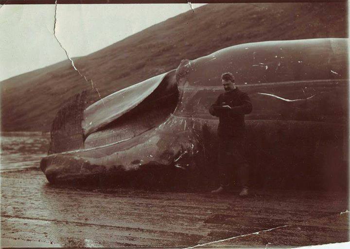
^{Statistician at work, counting whales. To quote from the FRAM, High North Research Centre for the Climate and Enviroment: Johan Hjort taking notes, probably at the whaling base in Mehamn early in the spring of 1901. He is standing in front of a North Atlantic right whale (Eubalaena glacialis). This species is currently endangered; only about 350 individuals remain, mostly along the east coast of the United States. Photo courtesy of Nils Lid Hjort.}

Counting fish or whales is just as easy as counting trees – apart from the facts that they are invisible and that they move, sometimes large distances. Also, they're not easy to mark, in the usual fashion.The Bravington-Skaug methods use the most steadfast of all marks, however, namely the DNA. Also, since they for good reasons can't catch the very same fish twice – (a) it would be unlikely, if they throw a marked fish back into the ocean, to find it again, and (b) it's very dead, anyway, since they needed drastic surgery to read off its DNA – so what they're occasionally able to do, via the DNA, is to ascertain degrees of close-kin-ness, for some of the pairs of fish. Cases looked for include parent-offspring, half-siblings, etc. Estimators for population abundance and spawning stock biomass can then be worked out, using precise probability models for such kinships. The relevant probabilities, modelled and estimated, via intricacies of mathematical and probabilistical demography, play the roles of multiplicative factors in some of the estimators.

In a little more detail, the close-kin mark-recapture machinery involves setting up the right versions of a log-pseudo-likelihood function, based on those close-kin pairs of fish one has managed to find in the data, of the type

\(\ell^*(\theta)=\sum_{i<j} \log P(K_{i,j}=k_{i,j,{{\rm obs}}}\mid\theta,z_i,z_j).\)

Here $\theta$ comprises the unknown parameters of the model, including the crucial parameter $N$, the total population size, and with relevant covariate information $z_i,z_j$ associated with the pair $(i,j)$. Part of the challenge is to arrive at relevant demographical-probabilistical formulae for the $P(K_{i,j}=k_{i,j}\mid\theta,z_i,z_j)$ part. This involves probability calculations, under sets of conditions, that are perhaps similar to, but rather more complicated, than the simpler ones tended to above.

One of the formulae Skaug pointed to, as part of this general setup, was indeed the statistical curiosum that Pr(your mother is alive) = 0.50. This is partly what caught my attention and curiosity, leading to the present FocuStat blog post. Skaug's formula is a special case inside a more general setup when sampling age-structured populations, involving also assumptions and models for mortality and birth rates; see Skaug (2017) and Førland (2019).

So when can the Close-Kin Mark-Recapture technology-estimation-machine work?

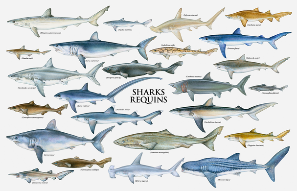
^{Lots 'o sharks – and though we can't really count them, very accurately, the close-kin mark-recapture methods are already in use to estimated species abundance and perhaps total biomass for several of them.} 

The Bravington-Skaug methods, for estimating population sizes and biomass from a single big haul of fish, are still hard to use, demanding sophisticated fine-reading and fine-tuning of several probabilities, as part of the general procedure. In one of the talks I've listened to the number of people in the world who can accurately and successfully apply the general machinery was cautiously estimated to $\widehat N_0=4$, but that number is expected to increase monotonically over time. Also, more theory needs to be developed regarding the precision of the estimates, perhaps involving sandwich variance matrices via pairwise pseudo-log-likelihoods, and spatial-temporal U-statistics. Those are tall orders, but in fifty years lots of significant stock assessments will exploit these close-kin mark-recapture methodologies, with heavy components of both technology and hard-core statistics, and most likely in combination with other information and assessments.

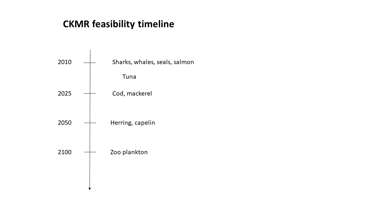
Skaug has sent me the following "feasibility timeline" for the close-kin mark-recapture methodology. So watch out, cod & mackerel, you'll be counted and assessed, with still better tools for marine sources management, over the years to come.

Footnotes

A. My little story above has been phrased in terms of mothers and daughters, but may of course be re-told using Turgenevian terms instead. The point is that women and men famously do not have identical lifelength distributions; the women tend to live longer, and in many societies and eras more boys have died early on than girls. But now both women and men live longer lives than before, with various demographic consequences. In connection with writing out my FocuStat blog story on Overdispersed and Markovian Children, I learned that for the first time in ages & ages, Norway now has more men than women.

B. Brage Frøland, one of Skaug's talented students, has in his June 2019 master's thesis generalised the $p=0.50$ result to certain formulae, under certain model conditions, involving birth and mortality rates.

C. I understand from various comments that Bravington and Skaug acknowledge crucial input from Tore Schweder, regarding the initial ideas behind the close-kin mark-recapture apparatus. Among these intial insights was that the amount and degrees of close-kin relationships found in a sample depend on the size of the population, and that this could be developed into usable formulae via probability models and DNA reading technology. I do believe these methods, suitably finessed and extended, will turn out to be exceedingly useful and important in the decades to come.

D. My blog post has attempted to make you think not only about your mother and the sequence of mothers before her, but about the prospect of combining cutting edge DNA technology with ambitious close-kin probability theory and sampling plans and statistical hard-core estimation theory to assess marine populations – from sharks and whales to cod and herring (and even more, over time). Før skal Hav og grommen Hval ham prise, Samt og Tanteyen, som løber Leyen, Steenbid og Seyen og Torsk og Skreyen! Og Niise! There are still other abundance assessment machineries, of course, partly using other technologies, and it appears important and viable to combine these diverse sources of information. A natural tool here would be the II-CC-FF machinery of Cunen and Hjort (2019) (independent inspection; confidence conversion; focused fusion).

E. I should think also Johan Hjort would've appreciated & applauded these modern methods, combining contextual understanding and modelling of fish populations, taking year-classes into the equations, combined with hard-core technology and statistical machineries. As Olav Kjesbu and Vera Schwach write, in a retrospective essay: "Johan Hjort: a marine research pioneer whose ideas still hold water: One hundred fifty years have passed since the birth of Johan Hjort (1869-1948). Best remembered for his groundbreaking theory from 1914 on the natural fluctuations of fish stocks, Hjort paved the way for materials and methods that are used to this day, not least in climate studies."

References

Borgan, Ø., Keilman, N. (2019). Do Japanese and Italian women live longer than women in Scandianvia? European Journal of Population, 35, 87-99.

Bravington, M., Grewe, P.M., Davies, C.R. (2016). Absolute abundance of Southern bluefin tuna estimated by close-kin mark-recapture. Nature Communications 7.

Bravington, M., Skaug, H.J., Anderson, E.C. (2016). Close-kin mark-recapture. Statistical Science, 2, 259-274.

Buckland, S.T., Morgan, B.J.T. (2016). Fifty-year anniversary of papers by Cormack, Jolly and Seber. Statistical Science, 31, 141.

Cunen, C., Hjort, N.L. (2018). Whales, Politics, and Statisticians. FocuStat Blog Post.

Cunen, C., Hjort, N.L. (2019). Combining information across diverse sources: the II-CC-FF paradigm. Technical report, Department of Mathematics, University of Oslo; submitted for publication.

Førland, B. (2019). Close-Kin Mark-Recapture Models. Master's Thesis in Statistics, University of Bergen.

Hermansen, G., Hjort, N.L., Kjesbu, O.S. (2016). Recent advances in statistical methodology applied to the Hjort liver index time series (1859-2012) and associated influential factors. Canadian Journal of Fisheries and Aquatic Sciences 73, 279-295.

><((((º>`·.¸¸.·´¯`·.¸.·´¯`·...¸><((((º>¸.
·´¯`·.¸. , . .·´¯`·.. ><((((º>`·.¸¸.·´¯`·.¸.·´¯`·...¸><((((º>

Hjort, N.L. (2016). Recruitment Dynamics and Stock Variability: The Johan Hjort Symposium, some personal reflections. FocuStat Blog Post. 

Hjort, N.L. (2018). Overdispersed and Markovian Children. FocuStat Blog Post.

Hoff, J.M., Hjort, N.L., Stenseth, N.C. (2020). A new class of methods for estimating population parameters from capture-mark-recapture experiments in open populations. (This is a paper we hope to write up, based on Hoff's extensive cand. real. thesis, 1983. The application concerns assessing population sizes, along with mortality and birth rates, for Microtus agrestis mice living in Finnish forests. Hoff and Hjort then generalised the classical Jolly-Seber methods to account for the clear fact that different mice had different probabilities of getting caught in Hoff's mousetraps.)

Kjesbu, O.S., Schwach, V. (2019). Johan Hjort: a marine research pioneer whose ideas still hold water. FRAM Centre essay.

Pinker, S. (2018). Enlightenment Now: The Case for Reason, Science, Humanism, and Progress.

Skaug, H.J. (2011). Allele-sharing methods for estimation of population size. Biometrics, 57, 750-756.

Skaug, H.J. (2017). The parent-offspring probability when sampling age-structured populations. Theoretical Populations Biology, 118, 20-26.

_{Let's trust these close-kinned fishermen not merely mark and capture but also release and recapture the Xiphiae gladii. From Barks' Flying Dutchman story, 1959.}